Chapter 07. Interactions
- so far, we have assumed that each predictor has an independent
association with the mean of the outcome
- now we will look at conditioning this estimate on another predictor using interactions
- fitting a model with interactions is easy, but understanding them can be harder
7.1 Building an interaction
- for examples, we will use information on the economy countries and geographic properties
data("rugged")

d <- rugged
d$log_gdp <- log(d$rgdppc_2000)
dd <- d[complete.cases(d$rgdppc_2000), ]
dd <- as_tibble(dd)
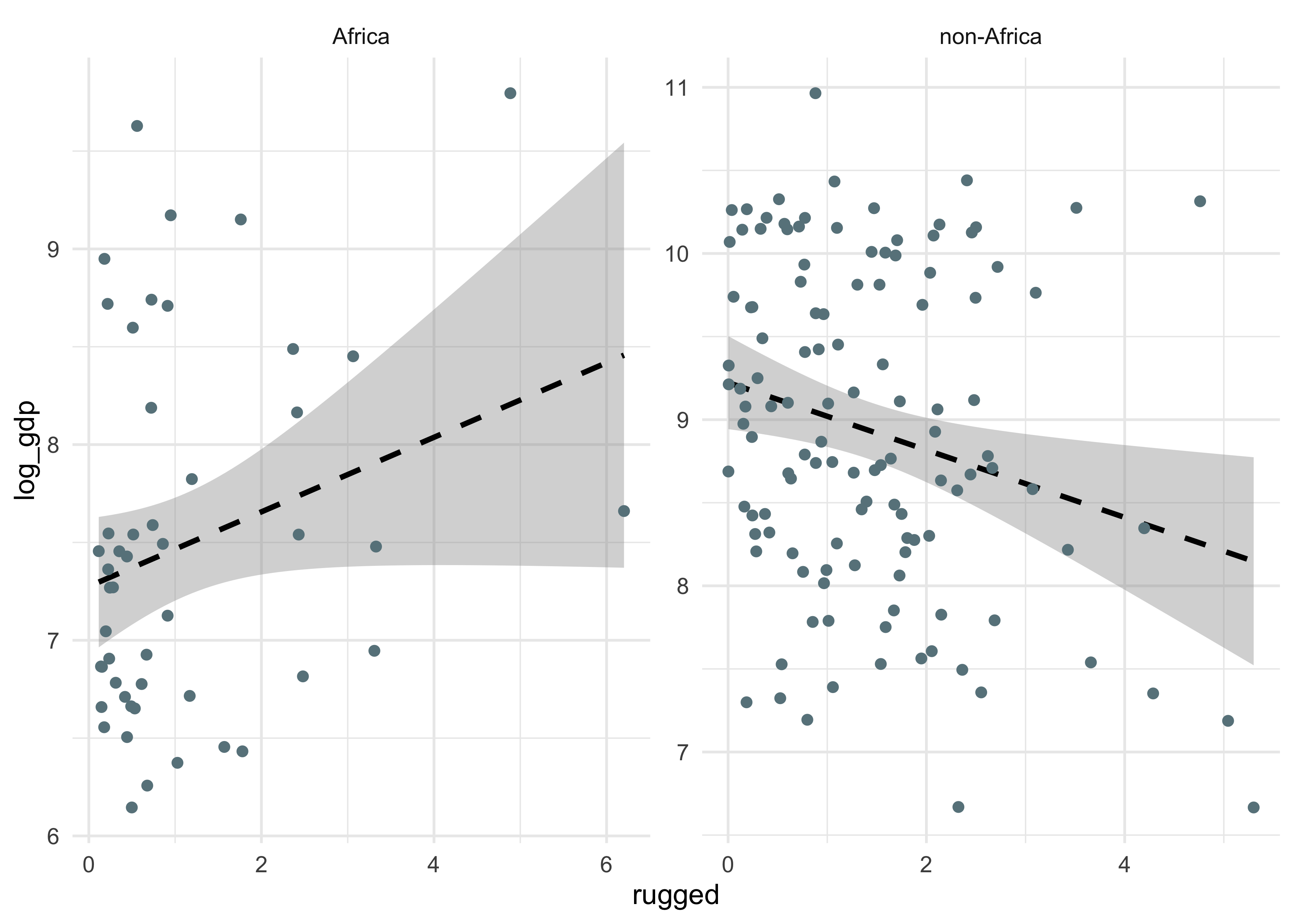
- one peculiarity is how the GDP of a country is associated to the
ruggedness of the terrain.
- the association is opposite for African and non-African countries
dd %>%
    mutate(is_africa = ifelse(cont_africa == 1, "Africa", "non-Africa")) %>%
    ggplot(aes(x = rugged, y = log_gdp)) +
    facet_wrap(~ is_africa, nrow = 1, scales = "free") +
    geom_smooth(method = "lm", formula = "y ~ x", color = "black", lty = 2) +
    geom_point(color = "lightblue4")
7.1.1 Adding a dummy variable doesn’t work
- two models to begin with:
- linear regression of log-GDP on ruggedness
- the same model with a dummy variable for the African nations
m7_3 <- quap(
    alist(
        log_gdp ~ dnorm(mu, sigma),
        mu <- a + bR*rugged,
        a ~ dnorm(8, 100),
        bR ~ dnorm(0, 1),
        sigma ~ dunif(0, 10)
    ),
    data = dd
)

m7_4 <- quap(
    alist(
        log_gdp ~ dnorm(mu, sigma),
        mu <- a + bR*rugged + bA*cont_africa,
        a ~ dnorm(8, 100),
        bR ~ dnorm(0, 1),
        bA ~ dnorm(0, 1),
        sigma ~ dunif(0, 10)
    ),
    data = dd
)

precis(m7_3)
#>              mean         sd       5.5%     94.5%
#> a     8.513367248 0.13533686  8.2970728 8.7296617
#> bR    0.002812495 0.07634323 -0.1191987 0.1248237
#> sigma 1.163054440 0.06307531  1.0622479 1.2638610
precis(m7_4)
#>              mean         sd       5.5%       94.5%
#> a      9.01583987 0.12505582  8.8159765  9.21570322
#> bR    -0.06479984 0.06337639 -0.1660875  0.03648787
#> bA    -1.43051778 0.16128018 -1.6882747 -1.17276091
#> sigma  0.95759964 0.05194951  0.8745743  1.04062499
compare(m7_3, m7_4)
#>          WAIC      SE    dWAIC      dSE    pWAIC       weight
#> m7_4 476.2639 15.2637  0.00000       NA 4.328950 1.000000e+00
#> m7_3 539.5791 13.3171 63.31523 15.05468 2.682669 1.783499e-14
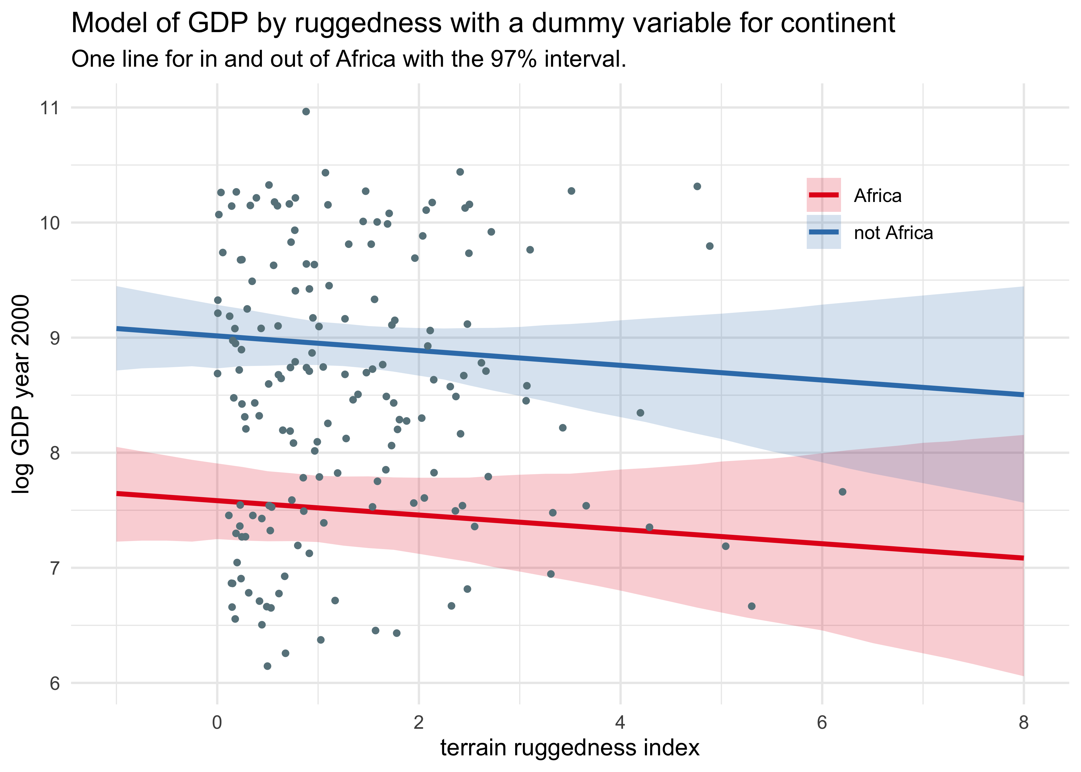
- plot the posterior distribution mean and intervals for African
countries and the rest
- we can see that the WAIC for the model with the dummy variable was lower because African countries tend to have lower GDP, not because it fit the different slope
rugged_seq <- seq(-1, 8, 0.25)

mu_notafrica <- link(m7_4, data = data.frame(cont_africa = 0,
                                             rugged = rugged_seq))
mu_africa <- link(m7_4, data = data.frame(cont_africa = 1,
                                          rugged = rugged_seq))

mu_notafrica_mean <- apply(mu_notafrica, 2, mean)
mu_notafrica_pi <- apply(mu_notafrica, 2, PI, prob = 0.97) %>% pi_to_df()

mu_africa_mean <- apply(mu_africa, 2, mean)
mu_africa_pi <- apply(mu_africa, 2, PI, prob = 0.97) %>% pi_to_df()

bind_rows(
    tibble(cont_africa = "not Africa",
           rugged = rugged_seq,
           mu = mu_notafrica_mean) %>%
        bind_cols(mu_notafrica_pi),
    tibble(cont_africa = "Africa",
           rugged = rugged_seq,
           mu = mu_africa_mean) %>%
        bind_cols(mu_africa_pi)
) %>%
    ggplot(aes(x = rugged)) +
    geom_ribbon(aes(ymin = x2_percent, ymax = x98_percent, fill = cont_africa),
                alpha = 0.2, color = NA) +
    geom_line(aes(y = mu, color = cont_africa), size = 1.1) +
    geom_point(data = dd, aes(y = log_gdp), size = 1, color = "lightblue4") +
    scale_color_brewer(palette = "Set1") +
    scale_fill_brewer(palette = "Set1") +
    theme(legend.position = c(0.8, 0.8)) +
    labs(x = "terrain ruggedness index",
         y = "log GDP year 2000",
         color = NULL, fill = NULL,
         title = "Model of GDP by ruggedness with a dummy variable for continent",
         subtitle = "One line for in and out of Africa with the 97% interval.")
7.1.2 Adding a linear interaction does work
- we have just used the model below:
$$ Y_i \sim \text{Normal}(\mu_i, \sigma) $$ $$ \mu_i = \alpha + \beta_R R_i + \beta_A A_i $$
- now we want to allow the relationship of $Y$ and $R$ to vary as
a function of $A$
- add in $\gamma$ as a placeholder for another linear function that defines the slope between GDP and ruggedness
- this is the linear interaction effect
- explicitly modeling that the slope between GDP and ruggedness is conditional upon whether or not a nation is in Africa
$$ Y_i \sim \text{Normal}(\mu_i, \sigma) $$ $$ \mu_i = \alpha + \gamma_i R_i + \beta_A A_i $$ $$ \gamma_i = \beta_R + \beta_{AR}A_i $$
- rearranging the above formula results in the following
$$ \mu_i = \alpha + \beta_R R_i + \beta_{AR} A_i R_i + \beta_A A_i $$
- fit the model using
quap()like normal
m7_5 <- quap(
    alist(
        log_gdp ~ dnorm(mu, sigma),
        mu <- a + gamma*rugged + bA*cont_africa,
        gamma <- bR + bAR*cont_africa,
        a ~ dnorm(8, 100),
        c(bA, bR, bAR) ~ dnorm(0, 1),
        sigma ~ dunif(0, 10)
    ),
    data = dd
)

precis(m7_5)
#>             mean         sd       5.5%       94.5%
#> a      9.1836228 0.13642358  8.9655916  9.40165401
#> bA    -1.8460606 0.21849326 -2.1952550 -1.49686613
#> bR    -0.1843913 0.07569178 -0.3053614 -0.06342126
#> bAR    0.3482859 0.12750672  0.1445055  0.55206624
#> sigma  0.9333055 0.05067821  0.8523120  1.01429910
plot(precis(m7_5))
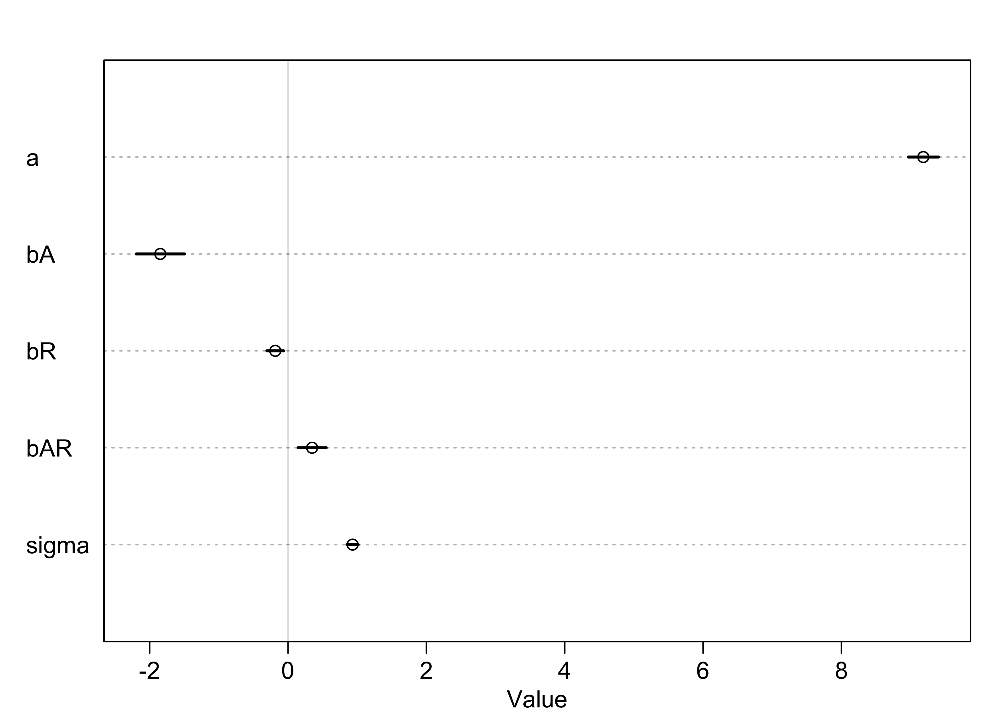
- the new model is far better than the previous two
compare(m7_3, m7_4, m7_5)
#>          WAIC       SE     dWAIC     dSE    pWAIC       weight
#> m7_5 469.7522 15.18797  0.000000      NA 5.359607 9.603456e-01
#> m7_4 476.1263 15.22849  6.374185  6.1519 4.269052 3.965435e-02
#> m7_3 539.6364 13.22767 69.884269 15.2575 2.715930 6.415809e-16
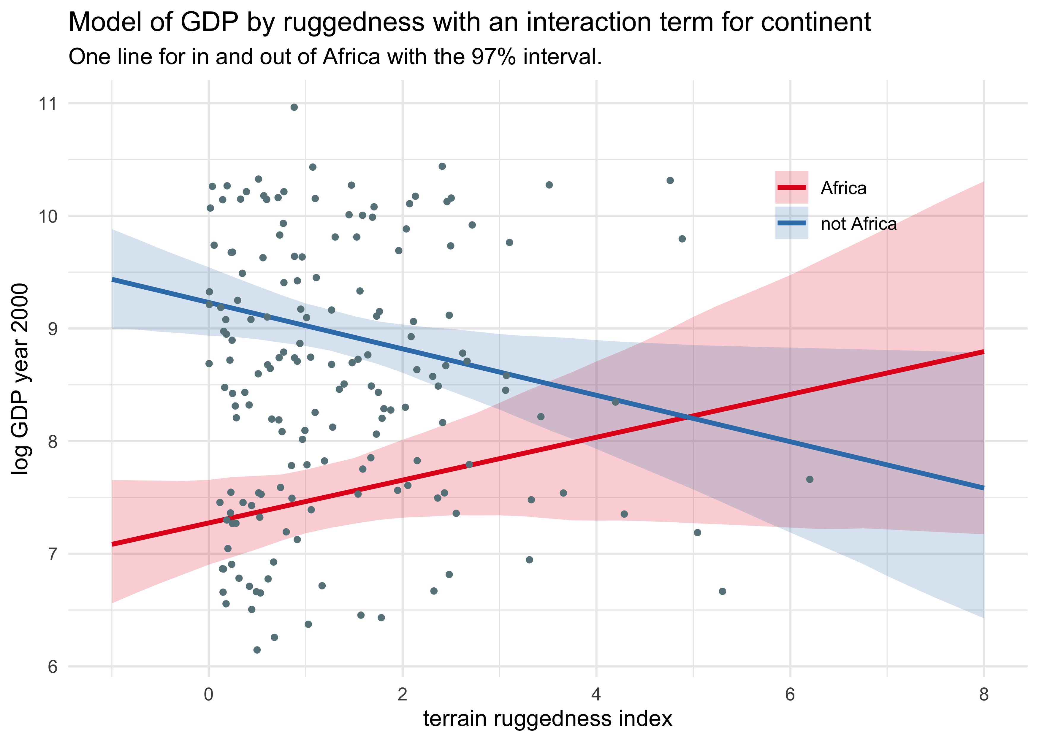
7.1.3 Plotting the interaction
- nothing new, just make two plots, one for African and one for non-African
rugged_seq <- seq(-1, 8, 0.25)

mu_africa <- link(m7_5,
                  data = data.frame(cont_africa = 1, rugged = rugged_seq))
mu_africa_mean <- apply(mu_africa$mu, 2, mean)
mu_africa_pi <- apply(mu_africa$mu, 2, PI, prob = 0.97) %>% pi_to_df()

mu_notafrica <- link(m7_5,
                     data = data.frame(cont_africa = 0, rugged = rugged_seq))
mu_notafrica_mean <- apply(mu_notafrica$mu, 2, mean)
mu_notafrica_pi <- apply(mu_notafrica$mu, 2, PI, prob = 0.97) %>% pi_to_df()

bind_rows(
    tibble(cont_africa = "not Africa",
           rugged = rugged_seq,
           mu = mu_notafrica_mean) %>%
        bind_cols(mu_notafrica_pi),
    tibble(cont_africa = "Africa",
           rugged = rugged_seq,
           mu = mu_africa_mean) %>%
        bind_cols(mu_africa_pi)
) %>%
    ggplot(aes(x = rugged)) +
    geom_ribbon(aes(ymin = x2_percent, ymax = x98_percent, fill = cont_africa),
                alpha = 0.2, color = NA) +
    geom_line(aes(y = mu, color = cont_africa), size = 1.1) +
    geom_point(data = dd, aes(y = log_gdp), size = 1, color = "lightblue4") +
    scale_color_brewer(palette = "Set1") +
    scale_fill_brewer(palette = "Set1") +
    theme(legend.position = c(0.8, 0.8)) +
    labs(x = "terrain ruggedness index",
         y = "log GDP year 2000",
         color = NULL, fill = NULL,
         title = "Model of GDP by ruggedness with an interaction term for continent",
         subtitle = "One line for in and out of Africa with the 97% interval.")

7.1.4 Interpreting the interaction estimate
- helpful to plot implied predictions
- often only numbers are reported, though they are difficult to
interpret because:
- the parameters have different meanings because they are no longer independent
- it is very difficult to propagate the uncertainty when trying to understand multiple parameters simultaneously
- remember that the interaction term $y$ is a distribution
- we can sample from it for African and non-African countries
post <- extract.samples(m7_5)
gamma_africa <- post$bR + post$bAR*1
gamma_notafrica <- post$bR + post$bAR*0

tibble(Africa = gamma_africa,
       `not Africa` = gamma_notafrica) %>%
    pivot_longer(everything()) %>%
    ggplot(aes(x = value)) +
    geom_density(aes(fill = name, color = name), alpha = 0.3) +
    scale_color_brewer(palette = "Set1") +
    scale_fill_brewer(palette = "Set1") +
    labs(x = "posterior estimates of gamma",
         y = "probability density",
         title = "Probability distribution for the estimates of gamma",
         subtitle = "Gamma is the slope of the interaction term")
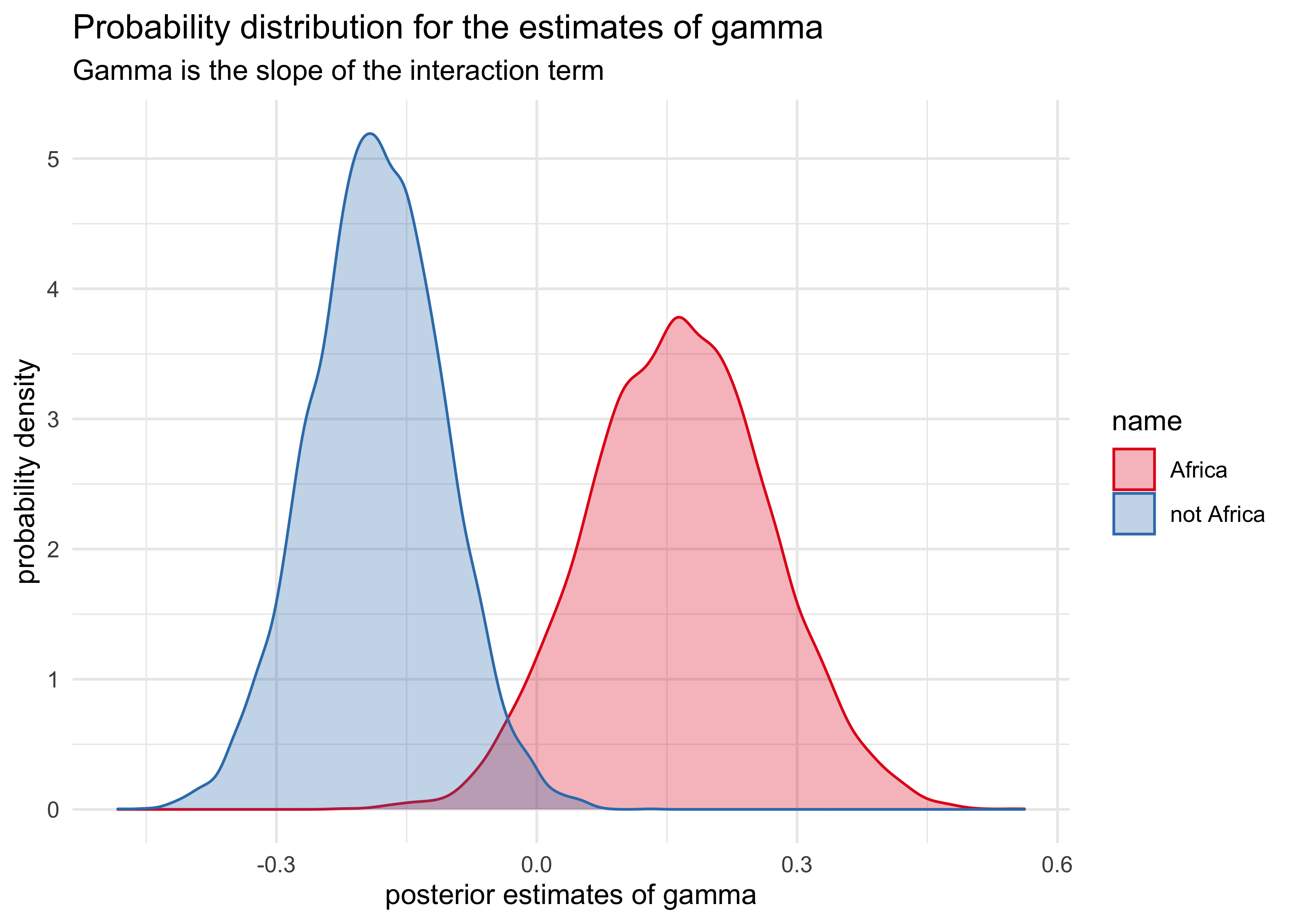
- can use these estimates like normal:
- e.g.: what is the probability that the slope within Africa is less than the slope outside of Africa
# The probability that the slope within Africa is less than that outside.
sum(gamma_africa < gamma_notafrica) / length(gamma_africa)
#> [1] 0.0031
7.2 Symmetry of the linear interaction
- the interaction term we have fit has two different phrasings:
- “How much does the influence of ruggedness (on GDP) depend upon whether the nation is in Africa?”
- How much does the influence of being in Africa (on GDP) depend upon ruggedness?
- the model interprets these as the same statement
7.2.1 Buridan’s interaction
- the model’s formula can be rearranged
- the same model can be reformulated to group the $A_i$ terms together
- shows that linear interactions are symmetric
$$ Y_i \sim \text{Normal}(\mu_i, \sigma) $$ $$ \mu_i = \alpha + \gamma_i R_i + \beta_A A_i $$ $$ \gamma_i = \beta_R + \beta_{AR}A_i $$ $$ \ $$ $$ \mu_i = \alpha + (\beta_R + \beta_{AR}A_i) R_i + \beta_A A_i $$ $$ \mu_i = \alpha + \beta_R R_i + \beta_{AR}A_i R_i + \beta_A A_i $$ $$ \ $$ $$ \mu_i = \alpha + \beta_R R_i + (\beta_{AR} R_i + \beta_A) A_i $$ $$ $$
7.2.2 Africa depends upon ruggedness
- below is a plot of the reverse interpretation of the interaction
term
- the x-axis is now whether the country is in Africa
- the points are the ruggedness separated by high and low (using the median as the cut-off)
- the blue slope is the expected reduction in log GDP for a non-rugged terrain if it was moved to Africa
- for countries in very rugged terrains, the continent has little effect
q_rugged  <- range(dd$rugged)

mu_ruggedlo <- link(m7_5,
                    data = data.frame(rugged = q_rugged[1],
                                      cont_africa = 0:1))
mu_ruggedlo_mean <- apply(mu_ruggedlo$mu, 2, mean)
mu_ruggedlo_pi <- apply(mu_ruggedlo$mu, 2, PI) %>% pi_to_df()

mu_ruggedhi <- link(m7_5,
                    data = data.frame(rugged = q_rugged[2],
                                      cont_africa = 0:1))
mu_ruggedhi_mean <- apply(mu_ruggedhi$mu, 2, mean)
mu_ruggedhi_pi <- apply(mu_ruggedhi$mu, 2, PI) %>% pi_to_df()

bind_rows(
    tibble(rugged = "low",
           cont_africa = 0:1,
           name = "low",
           mu_rugged = mu_ruggedlo_mean) %>%
        bind_cols(mu_ruggedlo_pi),
    tibble(rugged = "high",
           cont_africa = 0:1,
           mu_rugged = mu_ruggedhi_mean) %>%
        bind_cols(mu_ruggedhi_pi)
) %>%
    ggplot(aes(x = cont_africa)) +
    geom_ribbon(aes(ymin = x5_percent, ymax = x94_percent,
                    fill = factor(rugged)), alpha = 0.2) +
    geom_line(aes(y = mu_rugged, color = factor(rugged))) +
    geom_jitter(
        data = dd,
        aes(x = cont_africa, y = log_gdp,
            color = ifelse(rugged < median(rugged), "low", "high")),
        alpha = 0.4, width = 0.03
    ) +
    scale_color_brewer(palette = "Set1") +
    scale_fill_brewer(palette = "Set1") +
    scale_x_continuous(breaks = c(0, 1), labels = c("not Africa", "Africa")) +
    labs(x = NULL,
         y  = "log GDP year 2000",
         fill = "ruggedness", color = "ruggedness",
         title = "Symmetric interpretation of the interaction term")
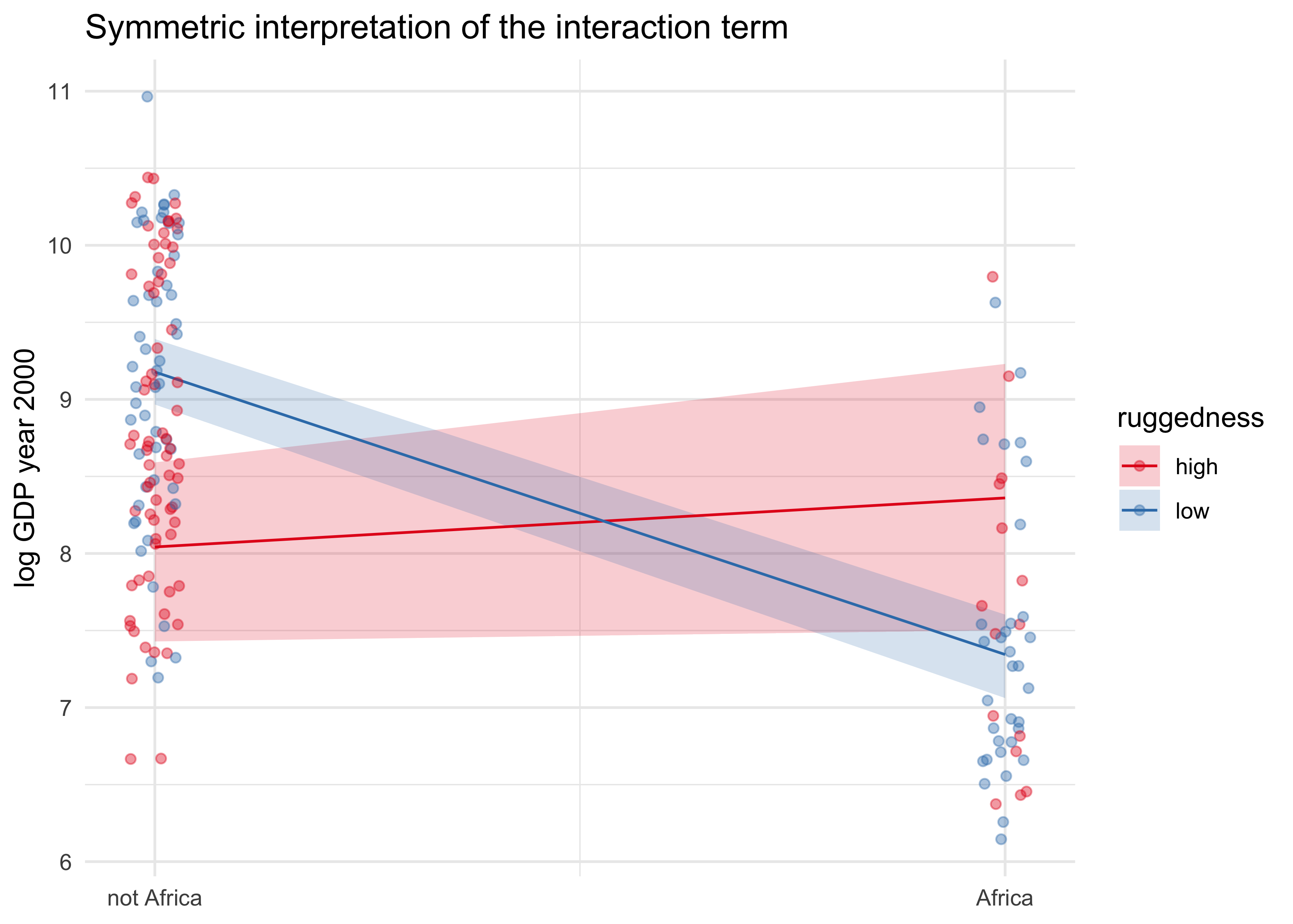
- it is simultaneously true that:
- the influence of ruggedness depends on the continent
- the influence of continent depends in the ruggedness
7.3 Continuous interactions
- interaction effects are difficult to interpret
- especially with only tables of posterior means and std. devs.
- we will look at using a triptych plot to understand these effects
- it is very important to center and standardize the predictors when using interactions
7.3.1 The data
- for examples we will use sizes of blooms from beds of tulips grown
in greenhouses with different soil and light
- we are interested in the interaction of light and water
data("tulips")
d <- as_tibble(tulips)
str(d)
#> tibble [27 × 4] (S3: tbl_df/tbl/data.frame)
#>  $ bed   : Factor w/ 3 levels "a","b","c": 1 1 1 1 1 1 1 1 1 2 ...
#>  $ water : int [1:27] 1 1 1 2 2 2 3 3 3 1 ...
#>  $ shade : int [1:27] 1 2 3 1 2 3 1 2 3 1 ...
#>  $ blooms: num [1:27] 0 0 111 183.5 59.2 ...
7.3.2 The un-centered models
- the author demonstrates fitting and interpreting the models without centering the data
7.3.3 Center and re-estimate
d$shade_c <- d$shade - mean(d$shade)
d$water_c <- d$water - mean(d$water)
- fit two models for predicting number of blooms with water and shade
- the second model includes their interactions
- starting places for the fitting are provided because the priors are very flat
m7_8 <- quap(
alist(
blooms ~ dnorm(mu, sigma),
mu <- a + bW*water_c + bS*shade_c,
a ~ dnorm(130, 100),
c(bW, bS) ~ dnorm(0, 100),
sigma ~ dunif(0, 100)
),
data = d,
start = list(a = mean(d$blooms),
bW = 0, bS = 0,
sigma = sd(d$blooms))
)
m7_9 <- quap(
alist(
blooms ~ dnorm(mu, sigma),
mu <- a + bW*water_c + bS*shade_c + bWS*water_c*shade_c,
a ~ dnorm(130, 100),
c(bW, bS, bWS) ~ dnorm(0, 100),
sigma ~ dunif(0, 100)
),
data = d,
start = list(a = mean(d$blooms),
bW = 0, bS = 0, bWS = 0,
sigma = sd(d$blooms))
)
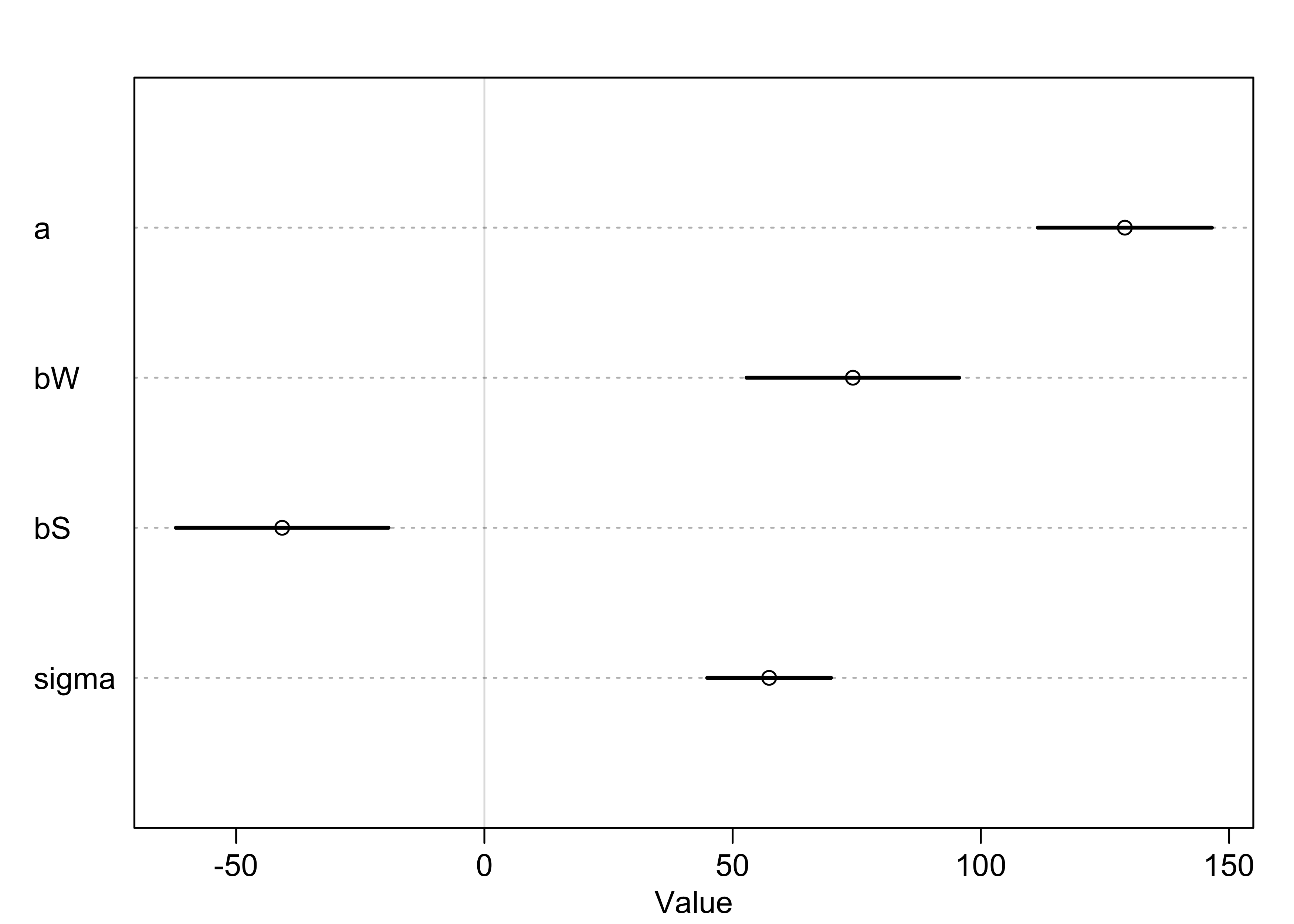
plot(precis(m7_8))
plot(precis(m7_9))
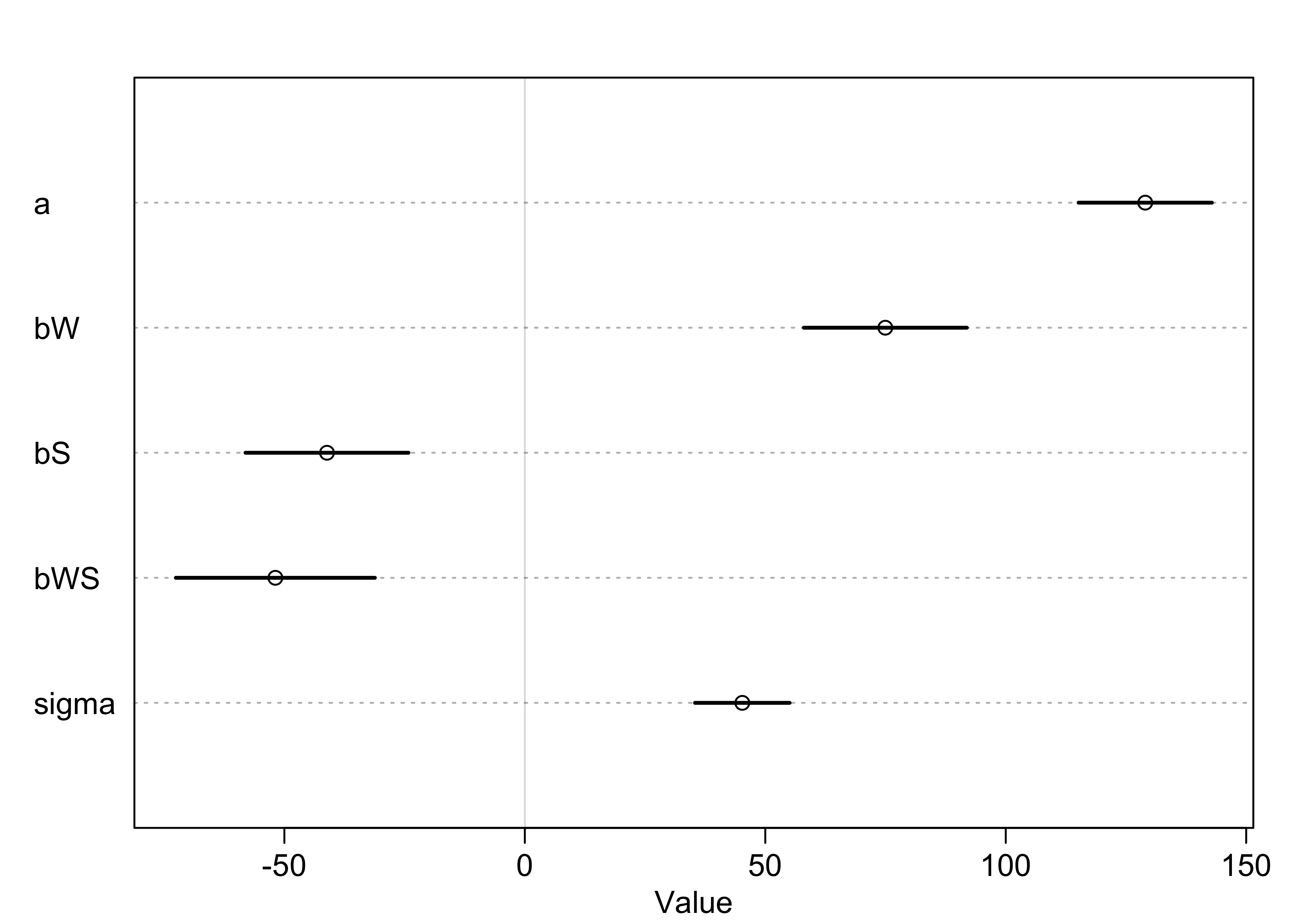
coeftab(m7_8, m7_9)
#>       m7_8    m7_9
#> a      129.00  129.01
#> bW      74.22   74.96
#> bS     -40.74  -41.14
#> sigma   57.35   45.22
#> bWS        NA  -51.87
#> nobs       27      27
compare(m7_8, m7_9)
#>          WAIC        SE    dWAIC      dSE    pWAIC     weight
#> m7_9 295.9624 10.252522  0.00000       NA 6.565320 0.99593805
#> m7_8 306.9664  9.254801 11.00404 8.473258 5.848144 0.00406195
- the main effects are the same between the two models
- if the predictors were not centered, the coefficient for shade in the model with the interaction would have been positive
- with the data centered, the intercept has meaning - it is the mean number of blooms
- interpretations of the estimates for the model with the interaction
term
m7_9:- $\alpha$: the expected value of blooms when both water and shade are at their average values (0 from centering)
- $\beta_W$: the expected change in blooms when water increases by 1 unit and shade is at its average value
- $\beta_S$: the expected change in blooms when shade increases by 1 unit and water is at its average value
- $\beta_{WS}$: the interaction term has multiple
interpretations:
- the expected change in the influence of water on blooms when increasing shade by one unit
- the expected change in the influence of shade on blooms when increasing water by one unit
7.3.4 Plotting implied predictions
- make a triptych plot to help understand interactions:
- plot the bivariate relationship between shade and blooms
- each of the 3 plots will show predictions for different values of water
shade_seq <- seq(-1, 1)

purrr::map(seq(-1, 1), function(w) {
    dt <- d[d$water_c == w, ]
    pred_data <- tibble(water_c = w, shade_c = shade_seq)
    mu <- link(m7_9, data = pred_data)
    pred_data %>%
        mutate(mu_mean = apply(mu, 2, mean)) %>%
        bind_cols(apply(mu, 2, PI) %>% pi_to_df())
}) %>%
    bind_rows() %>%
    ggplot(aes(x = shade_c)) +
    facet_wrap(~ water_c) +
    geom_ribbon(aes(ymin = x5_percent, ymax = x94_percent), alpha = 0.2) +
    geom_line(aes(y = mu_mean)) +
    geom_point(data = d, aes(y = blooms)) +
    labs(x = "shade (centered)",
         y = "blooms",
         title = "Effect of amount of light on impact of shade on blooms",
         subtitle = "Each panel is a different level of light.")
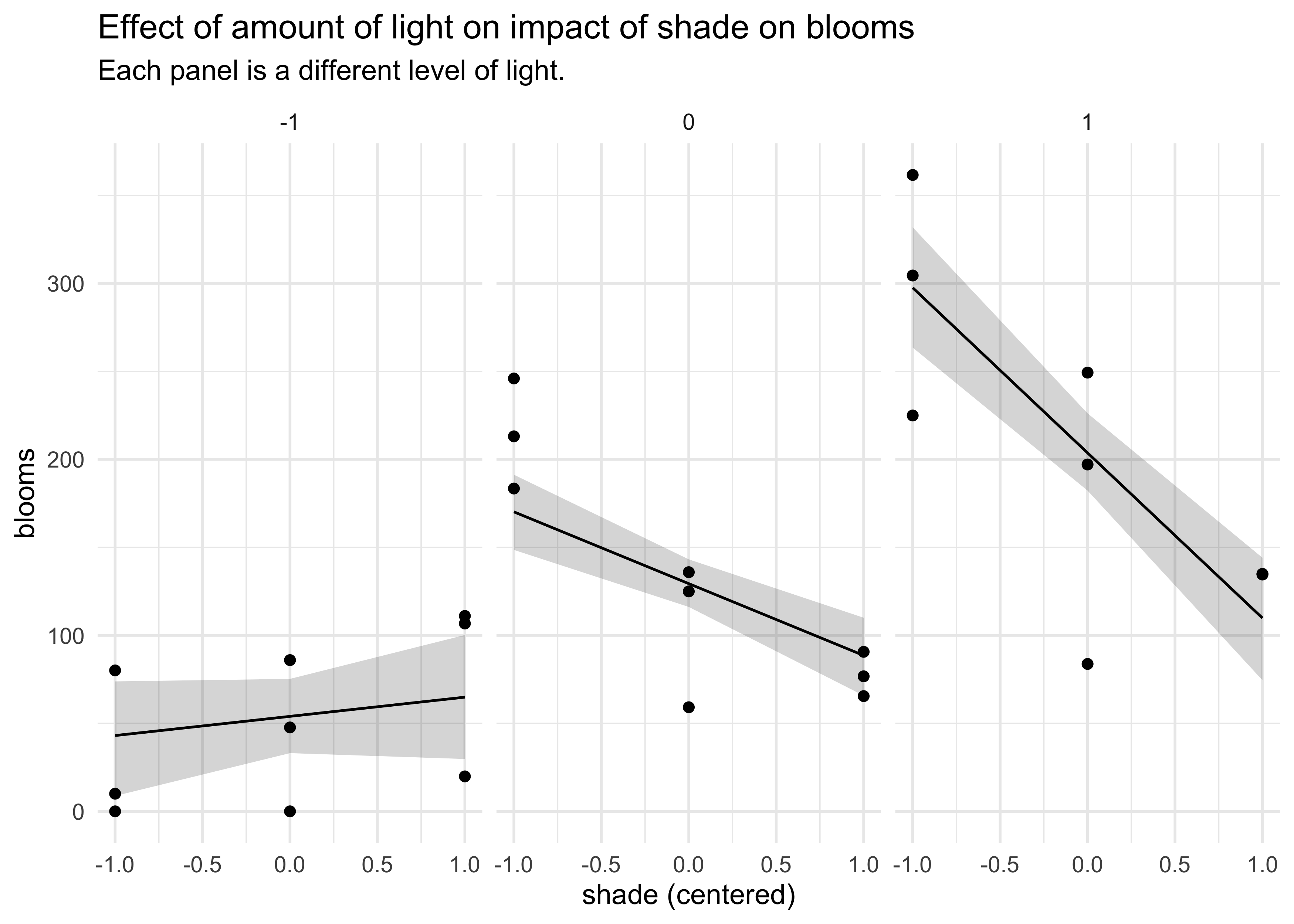
- this makes the interaction of the effects of shade and water easily
understandable
- plot on the left: when there is little water, the impact of shade is negligible
- plot on the right: when there is plenty of water, the shade has a larger impact on the number of blooms
7.4 Interactions in design formulas
- mathematical formula with an interaction between $x$ and $z$:
$$ y_i \sim \text{Normal}(\mu_i, \sigma) $$ $$ \mu_i = \alpha + \beta_x x_i + \beta_z z_i + \beta_{xz} x_i z_i $$
# Two equivalent model specifications.
m7_x <- lm(y ~ x + z + x*z, data = d)
m7_x <- lm(y ~ x*z, data = d)
- can also remove main effects by subtracting them out
- useful when we know a priori there is know effect of $z$ on $y$
m7_x <- lm(y ~ x + x*z - z, data = d)
- can use the following trick to see how R is interpreting a formula
x <- z <- w <- 1
colnames(model.matrix(~ x*z*w))
#> [1] "(Intercept)" "x"           "z"           "w"           "x:z"
#> [6] "x:w"         "z:w"         "x:z:w"
7.6 Practice
Hard.
7H1. Return to the data(tulips) example in the chapter. Now include the bed variable as a predictor in the interaction model. Don’t interact bed with the other predictors; just include it as a main effect. Note that bed is categorical. So to use it properly, you will need to either construct dummy variables or rather an index variable, as explained in Chapter 6.
# Add bed as a set of dummy variables.
# Bed "a" will be part of the intercept.
beds_dummy <- model.matrix(~ bed, data = d) %>%
    as.matrix() %>%
    as.data.frame() %>%
    set_names(paste0("bed_", letters[1:3]))
dd <- bind_cols(d, beds_dummy)

m_7h1 <- quap(
    alist(
        blooms ~ dnorm(mu, sigma),
        mu <- a + bW*water_c + bS*shade_c + bWS*water_c*shade_c + bb*bed_b + bc*bed_c,
        a ~ dnorm(130, 100),
        c(bW, bS, bWS, bb, bc) ~ dnorm(0, 50),
        sigma ~ dunif(0, 100)
    ),
    data = dd,
    start = list(a = mean(d$blooms),
                 bW = 0, bS = 0, bWS = 0,
                 bb = 0, bc = 0,
                 sigma = sd(d$blooms))
)

precis(m_7h1)
#>            mean        sd       5.5%     94.5%
#> a     103.19330 12.377857  83.411091 122.97550
#> bW     73.25915  9.184091  58.581194  87.93710
#> bS    -40.20735  9.166522 -54.857220 -25.55748
#> bWS   -50.18906 11.146401 -68.003157 -32.37496
#> bb     36.75643 17.277136   9.144226  64.36863
#> bc     41.14658 17.286259  13.519803  68.77336
#> sigma  39.52689  5.462863  30.796179  48.25760
7H2. Use WAIC to compare the model from 7H1 to a model that omits bed. What do you infer from this comparison? Can you reconcile the WAIC results with the posterior distribution of the bed coefficients?
compare(m_7h1, m7_9)
#>           WAIC        SE    dWAIC      dSE    pWAIC    weight
#> m_7h1 293.9713  9.720705 0.000000       NA 9.151898 0.7203902
#> m7_9  295.8641 10.292275 1.892796 6.531838 6.484775 0.2796098
It seems that the model that includes the bed information produced a better model. However, the improvement was not overwhelming as the difference in WAIC value is less than the standard error of the WAIC values and the weights are split about 75:25.
The beds seem to hold some information, perhaps some sort of batch effect. From the standard deviation and 89% interval of these coefficients, they are not very informative, given the other variables.
7H3. Consider again the data(rugged) data on economic development and terrain ruggedness, examined in this chapter. One of the African countries in that example, Seychelles, is far outside the cloud of other nations, being a rare country with both relatively high GDP and high ruggedness. Seychelles is also unusual, in that it is a group of islands far from the coast of mainland Africa, and its main economic activity is tourism.
One might suspect that this one nation is exerting a strong influence on the conclusions. In this problem, I want you to drop Seychelles from the data and re-evaluate the hypothesis that the relationship of African economies with ruggedness is different from that on other continents.
(a) Begin by using map to fit just the interaction model:
$$ y_i \sim \text{Normal}(\mu_i, \sigma) $$ $$ \mu_i = \alpha + \beta_A A_i + \beta_R R_i + \beta_{AR} A_i R_i $$
where $y$ is log GDP per capita in the year 2000 (log of
rgdppc_2000); $A$ is cont_africa, the dummy variable for being an
African nation; and $R$ is the variable rugged. Choose your own
priors. Compare the inference from this model fit to the data without
Seychelles to the same model fit to the full data. Does it still seem
like the effect of ruggedness depends upon continent? How much has the
expected relationship changed?
d <- rugged
d$log_gdp <- log(d$rgdppc_2000)
dd <- d[complete.cases(d$rgdppc_2000), ]
dd <- as_tibble(dd)

m7h3_1 <- quap(
    alist(
        log_gdp ~ dnorm(mu, sigma),
        mu <- a + bA*cont_africa + bR*rugged + bAR*cont_africa*rugged,
        a ~ dnorm(0, 20),
        c(bA, bR, bAR) ~ dnorm(0, 10),
        sigma ~ dunif(0, 10)
    ),
    data = dd
)

dd_noS <- dd %>% filter(country != "Seychelles")
m7h3_2 <- quap(
    alist(
        log_gdp ~ dnorm(mu, sigma),
        mu <- a + bA*cont_africa + bR*rugged + bAR*cont_africa*rugged,
        a ~ dnorm(0, 20),
        c(bA, bR, bAR) ~ dnorm(0, 10),
        sigma ~ dunif(0, 10)
    ),
    data = dd_noS
)

precis(m7h3_1)
#>             mean         sd       5.5%       94.5%
#> a      9.2229240 0.13798718  9.0023938  9.44345413
#> bA    -1.9470530 0.22451300 -2.3058681 -1.58823784
#> bR    -0.2027848 0.07647286 -0.3250032 -0.08056636
#> bAR    0.3931005 0.13005556  0.1852466  0.60095442
#> sigma  0.9327394 0.05058950  0.8518876  1.01359118
precis(m7h3_2)
#>             mean         sd        5.5%       94.5%
#> a      9.2223995 0.13689685  9.00361191  9.44118713
#> bA    -1.8810255 0.22532873 -2.24114429 -1.52090664
#> bR    -0.2024847 0.07586857 -0.32373733 -0.08123206
#> bAR    0.2970241 0.13828676  0.07601514  0.51803303
#> sigma  0.9253668 0.05033314  0.84492472  1.00580888
Removing Seychelles from the data reduced the MAP for the coefficient for continent $\beta_A$ and the interaction term $\beta_{AR}$. This suggests that Seychelles did have a relatively large impact on the effect from being in Africa and the interaction between being in Africa and terrain ruggedness.
(b) Now plot the predictions of the interaction model, with and without Seychelles. Does it still seem like the effect of ruggedness depends upon continent? How much has the expected relationship changed?
rugged_seq <- seq(-1, 8, 0.25)

plot_effect_of_africa <- function(mdl, original_data) {
    mu_africa <- link(mdl,
                      data = data.frame(cont_africa = 1,
                                        rugged = rugged_seq))
    mu_africa_mean <- apply(mu_africa, 2, mean)
    mu_africa_pi <- apply(mu_africa, 2, PI, prob = 0.97) %>% pi_to_df()

    mu_notafrica <- link(mdl,
                         data = data.frame(cont_africa = 0,
                                           rugged = rugged_seq))
    mu_notafrica_mean <- apply(mu_notafrica, 2, mean)
    mu_notafrica_pi <- apply(mu_notafrica, 2, PI, prob = 0.97) %>% pi_to_df()

    bind_rows(
        tibble(cont_africa = "not Africa",
               rugged = rugged_seq,
               mu = mu_notafrica_mean) %>%
            bind_cols(mu_notafrica_pi),
        tibble(cont_africa = "Africa",
               rugged = rugged_seq,
               mu = mu_africa_mean) %>%
            bind_cols(mu_africa_pi)
    ) %>%
        ggplot(aes(x = rugged)) +
        geom_ribbon(aes(ymin = x2_percent, ymax = x98_percent,
                        fill = cont_africa),
                    alpha = 0.2, color = NA) +
        geom_line(aes(y = mu, color = cont_africa), size = 1.1) +
        geom_point(data = original_data, aes(y = log_gdp),
                   size = 1, color = "lightblue4") +
        scale_color_brewer(palette = "Set1") +
        scale_fill_brewer(palette = "Set1") +
        theme(legend.position = c(0.8, 0.8)) +
        labs(x = "terrain ruggedness index",
             y = "log GDP year 2000",
             color = NULL, fill = NULL,
             title = "Model of GDP by ruggedness with an interaction term for continent",
             subtitle = "One line for in and out of Africa with the 97% interval.")
}

plot_effect_of_africa(m7h3_1, dd)
plot_effect_of_africa(m7h3_2, dd) +
    labs(subtitle = "One line for in and out of Africa with the 97% interval; without Seychelles.")
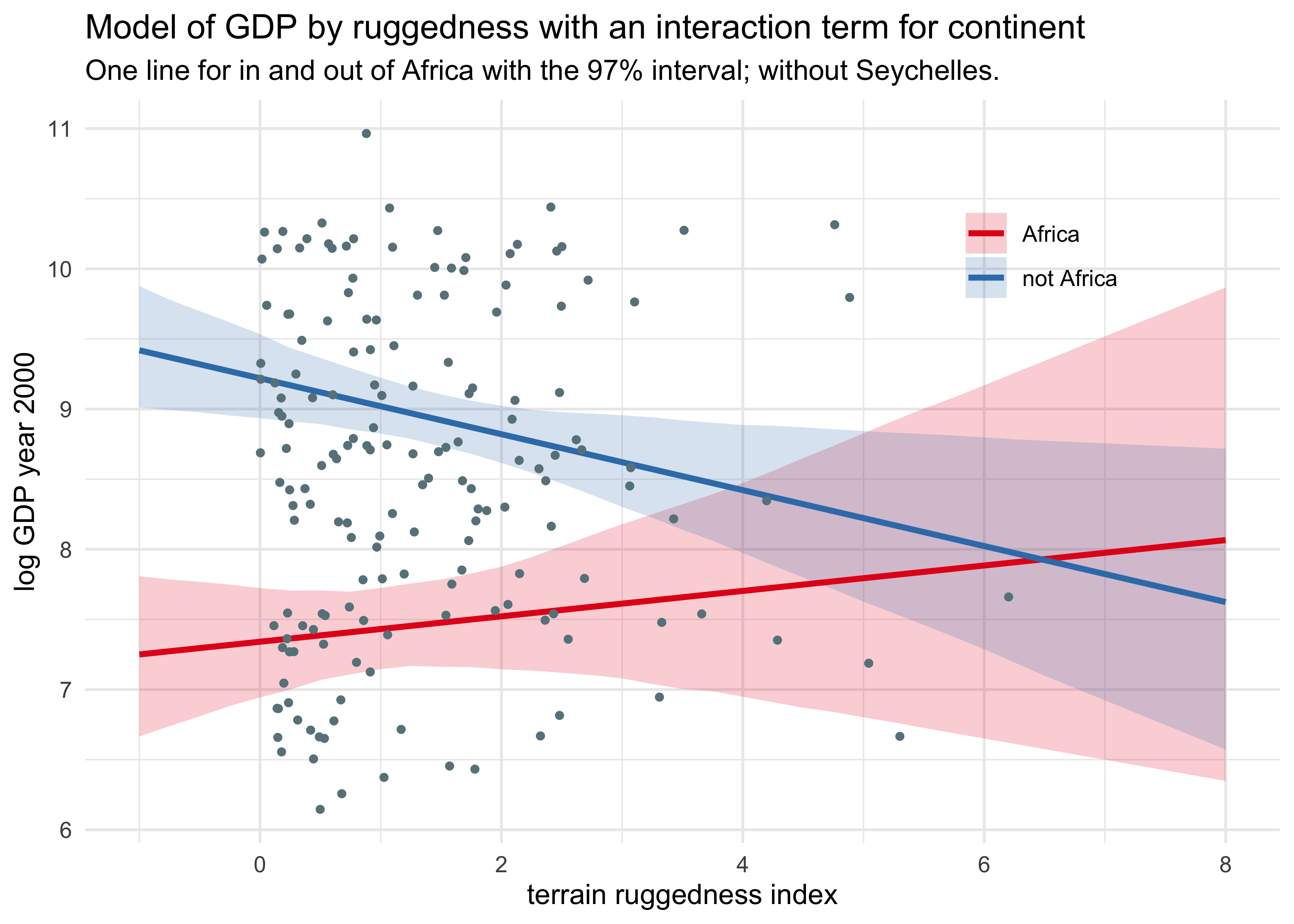
The angle of the red line decreases when Seychelles is removed. This suggests that Seychelles increased the impact of being in Africa as terrain ruggedness increased (and similarly for the symmetric interpretation of the interaction term).
Joshua Cook
Graduate Student
My research interests include cancer genetics and evolution. I also learning about programming and computer science in general.