Chapter 06. Overfitting Regularization And Information Criteria

Last updated on Jun 28, 2020 13 min read

simpler models tend to be preferred
- this chapter deals with comparing explanatory value of a model and its complexity
there are two general families:
- regularization
- use a scoring mechanism like information criteria
  - this chapter introduces information theory to cover these metrics

6.1 The problem with parameters

we should not just add all variables even if they are not correlated with each other
- adding parameters will generally improve the fit of the model to the data
- however, they can often predict worse on new data
- this is overfitting

6.1.1 More parameters always improve fit

overfitting: a model learns to much from a sample
for an example, we will use fake data on average brain volumes and body mass of hominid species

sppnames <- c("afarensis", "africanus", "habilis", "boisei",
              "rudolfensis", "ergaster", "sapiens")
brainvolcc <- c(438, 452, 612, 521, 752, 871, 1350)
masskg <- c(37.0, 35.5, 34.5, 41.5, 55.5, 61.0, 53.5)
d <- tibble(species=sppnames, brain=brainvolcc, mass=masskg)

we will use lm() instead of quap() for this part of the lesson as it is a bit faster and easier to use
- the main points will still apply
we will build increasingly complex models of this data
- the simplest is below, modelling brain volume of body size

$$ v_i \sim \text{Normal}(\mu_i, \sigma) $$ $$ \mu_i = \alpha + \beta_1 m_i $$

this model is fit below and the $R^2$ is calculated.

m6_1 <- lm(brain ~ mass, data = d)
1 - var(resid(m6_1)) / var(d$brain)  # R-squared

#> [1] 0.490158

consider 5 more models, each more complex with higher degree polynomials
- below is the formula for the 2nd-degree polynomial

$$ v_i \sim \text{Normal}(\mu_i, \sigma) $$ $$ \mu_i = \alpha + \beta_1 m_i + \beta_2 m_i^2 $$

m6_1 <- lm(brain ~ mass, data = d)
m6_2 <- lm(brain ~ mass + I(mass^2), data = d)
m6_3 <- lm(brain ~ mass + I(mass^2) + I(mass^3), data = d)
m6_4 <- lm(brain ~ mass + I(mass^2) + I(mass^3) + I(mass^4), data = d)
m6_5 <- lm(brain ~ mass + I(mass^2) + I(mass^3) + I(mass^4) + I(mass^5), data = d)
m6_6 <- lm(brain ~ mass + I(mass^2) + I(mass^3) + I(mass^4) + I(mass^5) + I(mass^6), data = d)

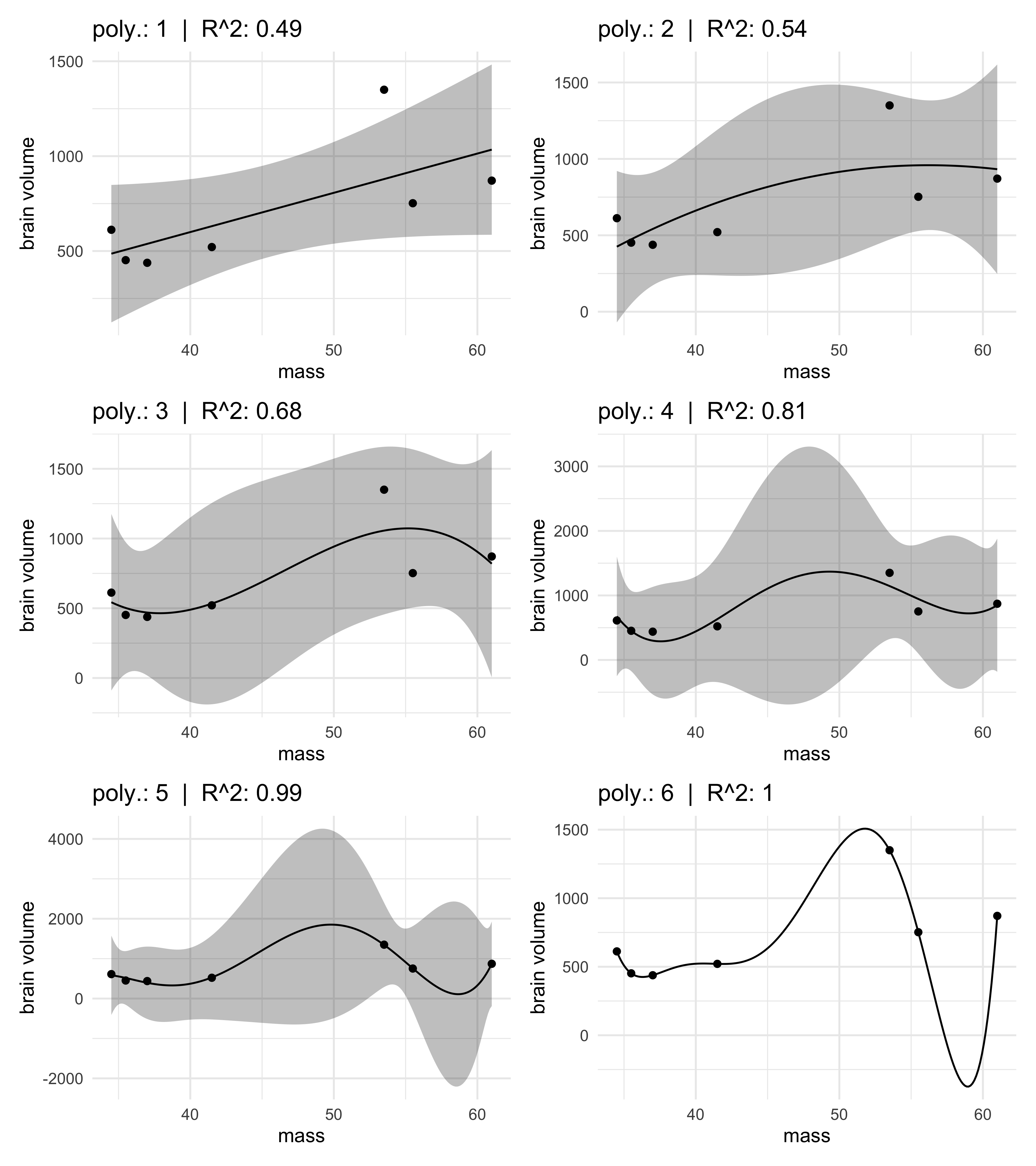
all of the fit models are shown against the original data, below
- the 5th order model has an $R^2 = 0.99$ and the 6th-order is 1
- the 6th order goes through every point
- there were enough parameters to assign one to each point of the data

fitted_plot <- function(fit, idx, ...) {
    mass_seq <- data.frame(mass = seq(min(fit$model$mass), max(fit$model$mass), 
                                      length.out = 200))
    predict(fit, newdata = mass_seq, interval = "confidence") %>%
        cbind(mass_seq) %>%
        ggplot() +
        geom_ribbon(aes(x = mass, ymin = lwr, ymax = upr), 
                    alpha = 0.3, color = NA) +
        geom_line(aes(x = mass, y = fit)) +
        geom_point(data = fit, aes(x = mass, y = brain)) +
        labs(title = glue("poly.: {idx}  |  R^2: {round(glance(fit)$r.squared, 2)}"),
             x = "mass", y = "brain volume")
}

list(m6_1, m6_2, m6_3, m6_4, m6_5, m6_6) %>%
    purrr::imap(fitted_plot) %>%
    patchwork::wrap_plots(ncol = 2)

#> Warning in qt((1 - level)/2, df): NaNs produced

#> Warning in max(ids, na.rm = TRUE): no non-missing arguments to max; returning -
#> Inf

6.1.2 Too few parameters hurts, too

too few parameters means the model has learned too little from the data

6.2 Information theory and model performance

(My notes on this section are relatively brief and focused on the main points application.)

must choose a target criterion of model performance
- this can be based on regularization or information criteria
then must choose a metric

6.2.1 Firing the weatherperson

accuracy depends on definition of the target
- two dimensions to accuracy:
  1. cost-benefit analysis: how much does it cost to be wrong?
  2. accuracy in context: how much can the model improve prediction?
we will use a weather prediction for example
- two weathermen make the following predictions for the probability of rain over the next 10 days in the same city
- the bottom row is the observed outcome

Day	1	2	3	4	5	6	7	8	9	10
Pred 1	1	1	1	0.6	0.6	0.6	0.6	0.6	0.6	0.6
Pred 2	0	0	0	0	0	0	0	0	0	0
Obs	R	R	R	S	S	S	S	S	S	S

the second prediction was correct more often than the first
- a higher hit rate (rate of correct predictions)

6.2.1.1 Costs and benefits

if we weight being caught in the rain as -5 and carrying an umbrella as -1:
- prediction 1 score: -7.2
- prediction 2 score: -15

6.2.1.2 Measuring accuracy

hit rate is not the only measure of accuracy
perhaps compute the probability of predicting the exact sequence of days:
- compute the probability of a correct prediction for each day
- multiply each probability together to get the joint probability of correctly predicting the sequence
- this is the joint likelihood for Bayes’ theorem
prediction 1 had a probability of $1^3 \times 0.4^7 \approx 0.005$ and prediction 2 had $0^3 \times 1^7 = 0$
- the 2nd prediction had no chance of being correct
- the 2nd prediction had a high average probability of being correct, it had a bad join probability of being correct
the joint probability is the likelihood in Bayes’ theorem
- the number of ways each event (sequence of rain and shine) could happen
now need to find a way to measure how incorrect the prediction is
- needs to account for how hard getting the correct prediction is

6.2.2 Information and uncertainty

How much is our uncertainty reduced by learning an outcome?
- how much is learned when we actually observe the day’s weather
- need a measure of uncertainty
information: the reduction in uncertainty derived from learning an outcome
need a way to quantify uncertainty inherent in a probability distribution
- use information entropy: “The uncertainty contained in a probability distribution is the average log-probability of an event.”

$$ H(p) = -E \log(p_i) = \ \sum_{i=1}^{n} p_i \log(p_i) $$

6.2.3 From entropy to accuracy

now need a measure of how far a model is from the target: divergence
divergence: “The additional uncertainty induced by using probabilities from one distribution to describe another distribution.”
- also known as Kullback-Leibler divergence (K-L divergence)
suppose the probabilities for two events are $p_1 = 0.3$, $p_2 = 0.7$
- if we instead believe these events have the probabilities $q_1 = 0.25$, $q_2 = 0.75$
- measure how much additional uncertainty has been introduced by using $q = {q_1, q_2}$ to estimate $p = {p_1, p_2}$?

$$ D_\text{KL}(p, q) = \sum_i p_i (\log(p_i) - \log(q_i)) = \sum_i p_i \log(\frac{p_i}{q_i}) $$

“the divergence is the average difference in log probability between the target (p) and model (q)”
- the difference between the entropy of the target $p$ and the cross entropy from using $q$ to predict $p$

6.2.4 From divergence to deviance

the above sections established the distance of a model from the target using K-L divergence
the remaining is to see how to estimate this divergence in a statistical model
so far, we have been comparing the model to the truth: compare true probability $p$ to estimated probability $q$
- the truth is not known in reality, though
- instead, we can compare two estimated $q$ and $r$, which causes the real probability $p$ to be subtracted out
  - cannot how far from the truth either model is, but we can tell which is further
we end up with a relative model fit as an estimate of K-L divergence
- we measure a model’s deviance:

$$ D(q) = -2 \sum_i \log(q_i) $$

the deviance of the estimates we have modeled in this course so far can be calculated:
- the $q$-values: use the MAP estimates to compute a log-probability of the observed data for each row
- sum and multiply by $-2$
- in R, this can be done by the logLik() function

-2 * logLik(m6_1)  # deviance

#> 'log Lik.' 94.92499 (df=3)

6.2.5 From deviance to out-of-sample

flaw with deviance: it will always improve with model complexity
- just like $R^2$
- the deviance on new data is really what we want

6.3 Regularization

can prevent overfitting by adding a regularization prior to a $\beta$ coefficient
- requires tuning to prevent both overfitting and underfitting
- a uniform or other broad prior may allow the model fitting algorithm to stray to extreme
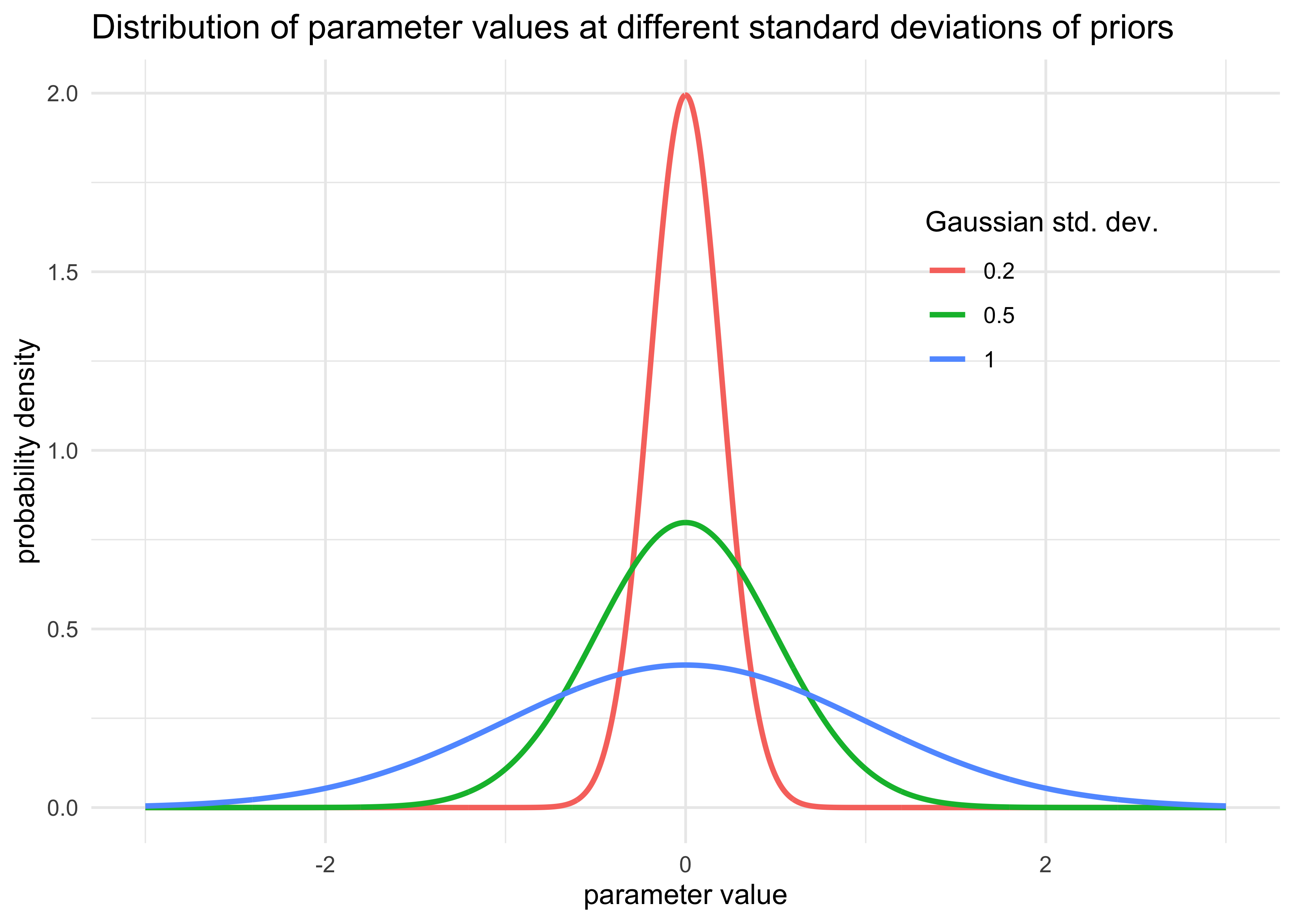
for example, consider the following Gaussian model (where $x$ is standardized)
- the prior for $\alpha$ is effectively uninformative
- the prior for $\beta$ is very strict

$$ y_i \sim \text{Normal}(\mu_i, \sigma) $$ $$ \mu_i = \alpha + \beta x_i $$ $$ \alpha \sim \text{Normal}(0, 100) $$ $$ \beta \sim \text{Normal}(0, 1) $$ $$ \sigma \sim \text{Uniform}(0, 10) $$

tibble(x = list(seq(-3, 3, length.out = 1e3)),
       std_dev = c(1, 0.5, 0.2)) %>%
    unnest(x) %>%
    mutate(prob_density = map2_dbl(x, std_dev, ~ dnorm(.x, mean = 0, sd = .y))) %>%
    ggplot(aes(x = x, y = prob_density, color = factor(std_dev))) +
    geom_line(size = 1) +
    theme(legend.position = c(0.8, 0.7)) +
    labs(x = "parameter value", 
         y = "probability density",
         title = "Distribution of parameter values at different standard deviations of priors",
         color = "Gaussian std. dev.")

the amount of regularization can be dewtermined using cross validation

6.4 Information criteria

Akaike information criterion provides an estimate of out-of-sample deviance:
- $p$ is the number of free parameters to be estimated

$$ \text{AIC} = D_\text{train} + 2p $$

AIC’s approximation is reliable when:
1. the priors are flat
2. the posterior distribution is approximately multivariate Gaussian
3. the sample size $N$ is much larger than the number of parameters $k$
because we rarely want to use flat priors, use DIC and WAIC more frequently:
- Deviance Information Criterion (DIC) accomidates informative priors but still assumes the posterior is multivariate Gaussian and $N \gg k$
- Widely Applicable Information Criterion (WAIC) is more general
  - makes no assumptions about the posterior

6.4.1 DIC

Deviance Information Criterion (DIC)
it is aware of informative priors
- by using the posterior distributions to calculate the deviance
assumes a multivariate Gaussian posterior distribution (like AIC)
- if a parameter in the posterior is highly skewed, DIC (and AIC) will give poor estimates

6.4.2 WAIC

Widely Applicable Information Criterion (WAIC)
does not require a multivariate Gaussian posterior
is often more accurate than DIC
- however, there are some models where defining WAIC is too difficult
- particularly where the points are not independent (line in time-series analysis)
it operates point-wise
- uncertainty in prediction is considered for each point in the data

6.4.3 DIC and WAIC as estimates of deviance

6.5 Using information criteria

this section discusses model comparison and model averaging:
- model comparison: using DIC/WAIC in combination with posterior predictive checks to each model
- model averaging:using DIC/WAIC to construct a posterior predictive distribution that uses what we know about relative accuracy of the models
  - “prediction averaging,” not averaging the estimates of multiple models

6.5.1 Model comparison

use the primate milk data for an example
- remove rows with missing information

data("milk")
d <- milk[complete.cases(milk), ] %>% janitor::clean_names()
d$neocortex <- d$neocortex_perc / 100

predict kilocalories per gram using neocortex size and the lagarithm of mass of the mother
- fit 4 different models with different combinations of these predictors
- also restrict the standard deviation of the final Gaussian $\sigma$ to be positive
  - estimate the logarithm of $\sigma$ and exponentiate it in the likelihood function
- all priors were left as flat

a_start <- mean(d$kcal_per_g)
sigma_start <- log(sd(d$kcal_per_g))

# Model kcal with no predictors (just an intercept)
m6_11 <- quap(
    alist(
        kcal_per_g ~ dnorm(a, exp(log_sigma))
    ),
    data = d,
    start = list(a = a_start,
                 log_sigma = sigma_start)
)

# Model kcal with neocortex
m6_12 <- quap(
    alist(
        kcal_per_g ~ dnorm(mu, exp(log_sigma)),
        mu <- a + bn*neocortex
    ),
    data = d,
    start = list(a = a_start,
                 bn = 0,
                 log_sigma = sigma_start)
)

# Model kcal with log(mass)
m6_13 <- quap(
    alist(
        kcal_per_g ~ dnorm(mu, exp(log_sigma)),
        mu <- a + bm*log(mass)
    ),
    data = d,
    start = list(a = a_start,
                 bm = 0,
                 log_sigma = sigma_start)
)

# Model kcal with neocortex and log(mass)
m6_14 <- quap(
    alist(
        kcal_per_g ~ dnorm(mu, exp(log_sigma)),
        mu <- a + bn*neocortex + bm*log(mass)
    ),
    data = d,
    start = list(a = a_start,
                 bn = 0,
                 bm = 0,
                 log_sigma = sigma_start)
)

6.5.1.1 Comparing WAIC values

can measure WAIC using the WAIC() function from the ‘rethinking’ package:
- first value is the WAIC
- lppd and pWAIC are used to calculate WAIC
- se is the standard error of the estimate from the sampling process

WAIC(m6_14)

#>        WAIC     lppd  penalty  std_err
#> 1 -15.39206 12.33699 4.640955 7.612751

get WAIC for all models
- the “weight” is roughly “an estiamte of the probability that the model will make the best predictions on new data, conditional on the set of models considered”

milk_models <- compare(m6_11, m6_12, m6_13, m6_14)
milk_models

#>             WAIC       SE    dWAIC      dSE    pWAIC     weight
#> m6_14 -15.862631 7.081823 0.000000       NA 4.406564 0.94839376
#> m6_11  -8.242263 4.517978 7.620368 6.802299 1.834151 0.02100133
#> m6_13  -8.136854 5.418315 7.725778 4.954064 2.874894 0.01992312
#> m6_12  -6.890172 4.251610 8.972459 7.101033 2.594300 0.01068179

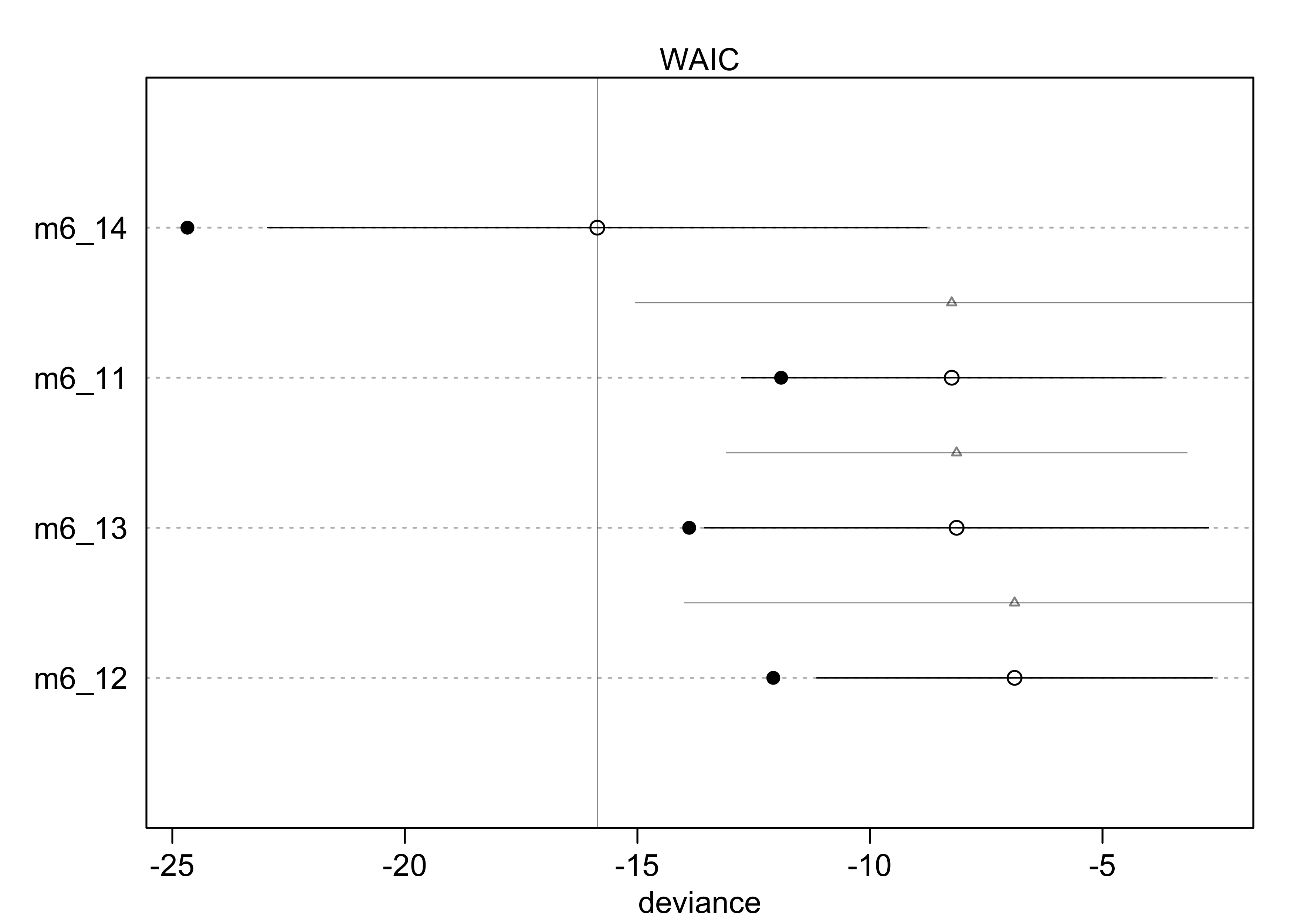
can plot the WAIC values and distributions
- unfilled points are the WAIC
- the SE of the difference between each WAIC and the top-ranke WAIC are the grey triangles

plot(milk_models, SE = TRUE, dSE = TRUE)

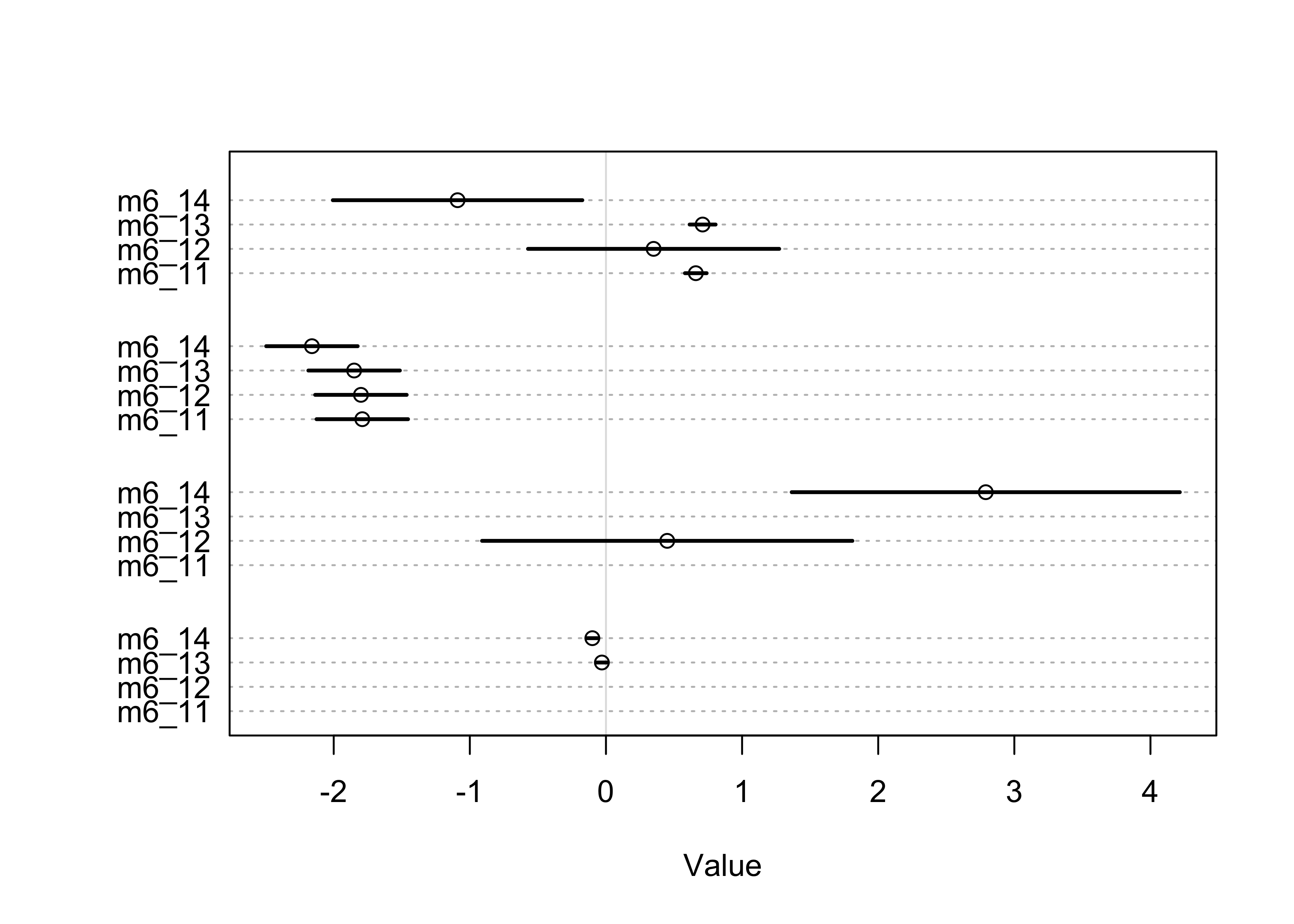
6.5.1.2 Comparing estimates

generally useful to compare parameter estimates of models
- can help to understand the WAIC values
- helps to understand the parameters to see if they remain stable across models

coeftab(m6_11, m6_12, m6_13, m6_14)

#>           m6_11   m6_12   m6_13   m6_14  
#> a            0.66    0.35    0.71   -1.09
#> log_sigma   -1.79   -1.80   -1.85   -2.16
#> bn             NA    0.45      NA    2.79
#> bm             NA      NA   -0.03   -0.10
#> nobs           17      17      17      17

plot(coeftab(m6_11, m6_12, m6_13, m6_14))

6.5.2 Model averaging

we want to use the weights from WAIC to generate predictions
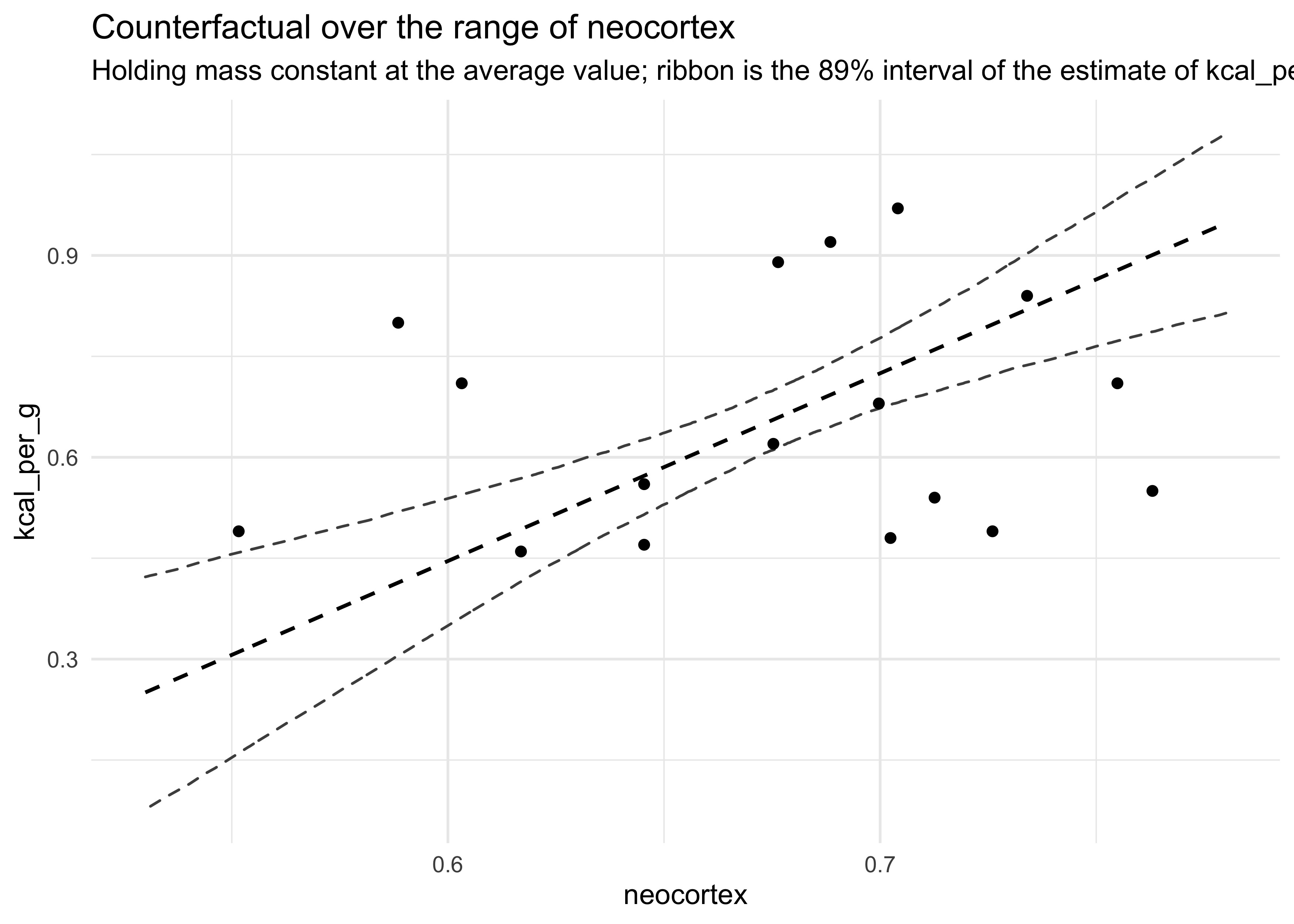
to review, start with simulating and plotting counterfactual predictions for m6_14 on the range of neocortex

nc_seq <- seq(0.53, 0.78, length.out = 1e3)
d_predict <- tibble(
    kcal_per_g = 0,
    neocortex = nc_seq,
    mass = 4.5
)

pred_m6_14 <- link(m6_14, data = d_predict)
mu <- apply(pred_m6_14, 2, mean)
mu_pi <- apply(pred_m6_14, 2, PI)

d_predict %>%
    mutate(mu_mean = mu) %>%
    bind_cols(pi_to_df(mu_pi)) %>%
    ggplot() +
    geom_ribbon(aes(x = neocortex, ymin = x5_percent, ymax = x94_percent),
                fill = NA, color = "grey30", lty = 2) +
    geom_line(aes(x = neocortex, y = mu_mean), lty = 2, size = 0.7) +
    geom_point(data = d, aes(x = neocortex, y = kcal_per_g)) +
    labs(x = "neocortex",
         y = "kcal_per_g",
         title = "Counterfactual over the range of neocortex",
         subtitle = "Holding mass constant at the average value; ribbon is the 89% interval of the estimate of kcal_per_g")

now we can compute and add model-averaged posterior predictions:
1. compute WAIC for each model
2. compute the weight for each model
3. compute linear model and simulated outcomes for each model
4. combine these values into an ensemble of predictions, using the model weights as proportions
this is automated by the ensemble() function from ‘rethinking’
- it uses link() and sim() to do the above process

milk_ensemble <- ensemble(m6_11, m6_12, m6_13, m6_14, data = d_predict)

mu_ens <- apply(milk_ensemble$link, 2, mean)
mu_pi_ens <- apply(milk_ensemble$link, 2, PI)

d_predict %>%
    mutate(mu_mean = mu,
           ensemble_mu = mu_ens) %>%
    bind_cols(pi_to_df(mu_pi) %>% set_names(c("m6_14_low", "m6_14_hi"))) %>%
    bind_cols(pi_to_df(mu_pi_ens) %>% set_names(c("ens_low", "end_hi"))) %>%
    ggplot(aes(x = neocortex)) +
    geom_ribbon(aes(ymin = m6_14_low, ymax = m6_14_hi),
                fill = NA, color = "grey30", lty = 2) +
    geom_line(aes(y = mu_mean), lty = 2, size = 0.7) +
    geom_ribbon(aes(ymin = ens_low, ymax = end_hi),
                fill = "black", color = NA, alpha = 0.2) +
    geom_line(aes(y = ensemble_mu), lty = 1, size = 0.7) +
    geom_point(data = d, aes(y = kcal_per_g)) +
    labs(x = "neocortex",
         y = "kcal_per_g",
         title = "Counterfactual over the range of neocortex",
         subtitle = 
"Holding mass constant at the avg.; dashed ribbon is the 89% interval of the estimate of kcal_per_g.
The shaded region and solid line are estimates using the ensemble approach.")

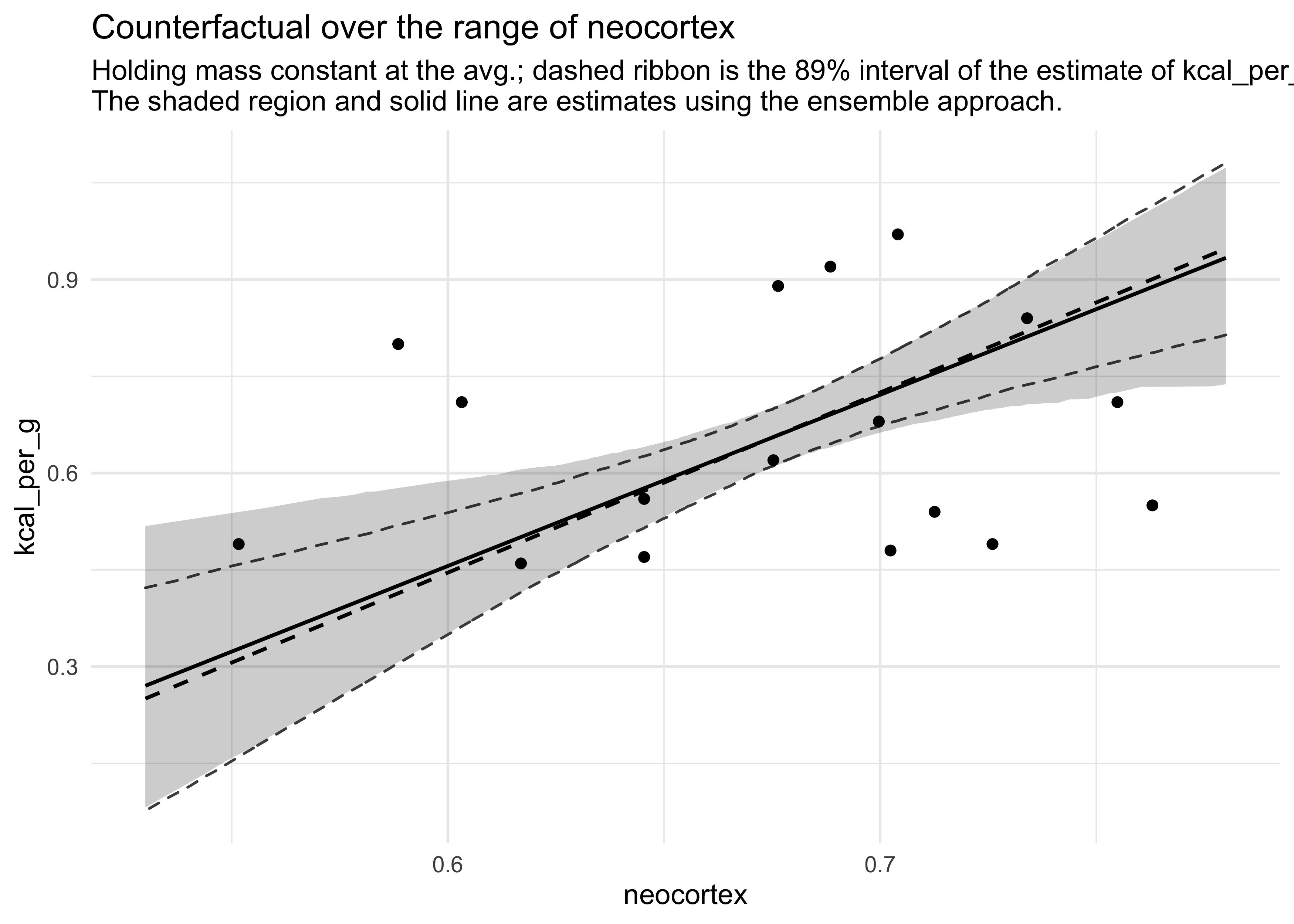
model averaging is a conservative approach
it communicates model uncertainty
will never make a predictor variable appear more influential than it already does in any single model

chapter_06