Chapter 14. Missing Data And Other Opportunities
- cover two common applications of Bayesian statistics:
- measurement error
- Bayesian imputation
14.1 Measurement error
- in the divorce and marriage data of states in the US, there was
error in the measured variables (marriage and divorce rates)
- this data can be incorporated into the model
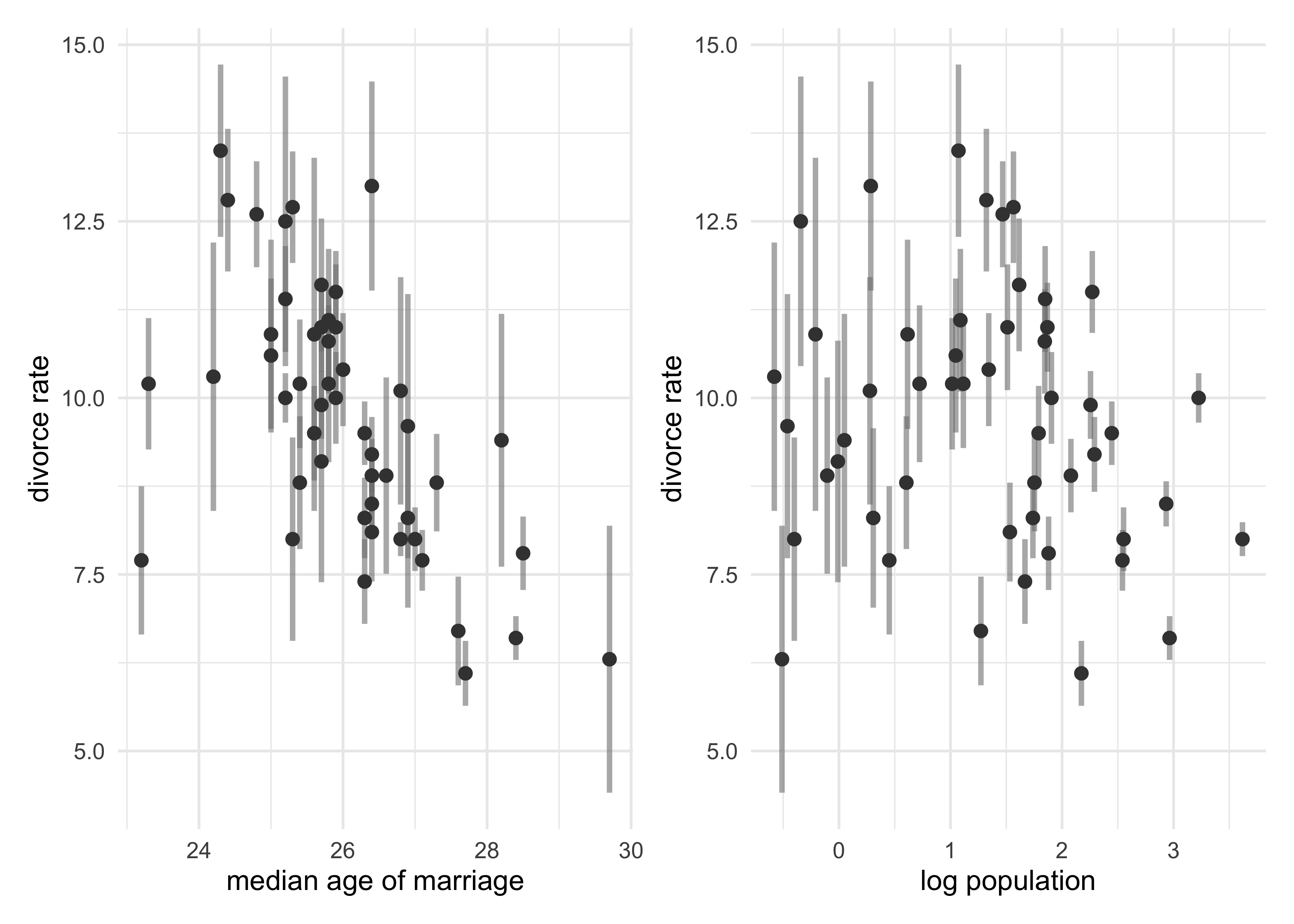
- the plot below shows the standard error in the measurement against median age of marriage and the population
- seems like smaller states have more error (smaller sample size)
# Load the data.
data("WaffleDivorce")
d <- as_tibble(WaffleDivorce) %>%
    janitor::clean_names()

p1 <- d %>%
    ggplot(aes(median_age_marriage, divorce)) +
    geom_linerange(aes(ymin = divorce - divorce_se, ymax = divorce + divorce_se),
                   size = 1, color = grey, alpha = 0.6) +
    geom_point(size = 2, color = dark_grey) +
    labs(x = "median age of marriage",
         y = "divorce rate")

p2 <- d %>%
    ggplot(aes(log(population), divorce)) +
    geom_linerange(aes(ymin = divorce - divorce_se, ymax = divorce + divorce_se),
                   size = 1, color = grey, alpha = 0.6) +
    geom_point(size = 2, color = dark_grey) +
    labs(x = "log population",
         y = "divorce rate")

p1 | p2
- makes sense to have the more certain estimates have more influence
on the regression
- many ad hoc methods for including this confidence as a weight in the analysis, but they leave out some data
14.1.1 Error on the outcome
Note: In the book, McElreath does not standardize the input variables for the new model (accounting for measurement error), but does standardize the variables in the previous model (not accounting for measurement error). Here I have standardized the input variables in both models and the differences from accounting for measurement error are not as astounding as reported in the book. I believe that my decision was correct and it does not remove the overall point of the section.
- to incorporate measurement error, replace the observed data for divorce rate with a distribution
- example:
- use a Gaussian distribution with a mean equal to the observed value and standard deviation equal to the measurement’s standard error
- define the distribution for each divorce rate:
- for each observed value $D_{\text{obs}, i}$ there will be one parameter $D_{\text{est}, i}$
- the measruement $D_{\text{obs}, i}$ is specified as a Gaussian distribution with the center of the estimate and standard deviation of the measurement
- can then estimate the plausible true values consistent with the observed data
$$ D_{\text{obs}, i} \sim \text{Normal}(D_{\text{est}, i}, D_{\text{SE}, i}) $$
- the model for the divorce rate $D$ as a linear function of age at
marriage $A$ and marriage rate $R$
- the first line is the likelihood for estimates
- the second line is the linear model
- the third line is the prior for estimates
- the main difference with this model compared to the normal ones
we have used previously is that the outcome is a vector of
parameters
- each outcome parameter also gets a second role as the unknown mean of another distribution to predict the observed measurement
- information will flow in both directions:
- the uncertainty in the measurement influences the regression parameters in the linear model
- the regression parameters in the linear model influence the uncertainty in the measurements
$$ D_{\text{est}, i} \sim \text{Normal}(\mu_i, \sigma) $$ $$ \mu_i = \alpha + \beta_A A_i + \beta_R R_i $$ $$ D_{\text{obs}, i} \sim \text{Normal}(D_{\text{est}, i}, D_{\text{SE}, i}) $$ $$ \alpha \sim \text{Normal}(0, 10) $$ $$ \beta_A \sim \text{Normal}(0, 10) $$ $$ \beta_R \sim \text{Normal}(0, 10) $$ $$ \sigma \sim \text{Cauchy}(0, 2.5) $$ $$ $$
- a few notes on the
map2stan()implementation of the above formula- turned off WAIC calculation because it will incorrectly compute
WAIC by integrating over the
div_estvalues - gave the model a starting point for
div_estas the observed values- this also tells it how many parameters it needs
- set the target acceptance rate from default 0.8 to 0.95 which causes Stan to “work harder” during warmup to improve the later sampling
- turned off WAIC calculation because it will incorrectly compute
WAIC by integrating over the
dlist <- d %>%
    transmute(div_obs = divorce,
              div_sd = divorce_se,
              R = scale_nums(marriage),
              A = scale_nums(median_age_marriage))

stash("m14_1", depends_on = "dlist", {
    m14_1 <- map2stan(
        alist(
            div_est ~ dnorm(mu, sigma),
            mu <- a + bA*A + bR*R,
            div_obs ~ dnorm(div_est, div_sd),
            a ~ dnorm(0, 10),
            bA ~ dnorm(0, 10),
            bR ~ dnorm(0, 10),
            sigma ~ dcauchy(0, 2.5)
        ),
        data = dlist,
        start = list(div_est = dlist$div_obs),
        WAIC = FALSE,
        iter = 5e3, warmup = 1e3, chains = 2, cores = 2,
        control = list(adapt_delta = 0.95)
    )
})
#> Loading stashed object.
- previously, the estimate for
bAwas about -1, now it is -0.5, but still comfortably negative- including measurement error reduced the estimated effect of another variable
precis(m14_1, depth = 1)
#> 50 vector or matrix parameters hidden. Use depth=2 to show them.

#>               mean        sd       5.5%      94.5%    n_eff     Rhat4
#> a      9.556418825 0.2044546  9.2376879  9.8812416 5002.159 1.0011619
#> bA    -1.242940436 0.3208026 -1.7527063 -0.7371894 3742.422 0.9999276
#> bR    -0.005569283 0.3420884 -0.5595417  0.5257439 3311.623 1.0000885
#> sigma  1.078827705 0.1961819  0.7872871  1.4068432 2199.206 1.0006505
precis(m14_1, depth = 2)
#>                  mean        sd      5.5%     94.5%    n_eff     Rhat4
#> div_est[1]  11.837345 0.6647418 10.788708 12.896255 5898.515 1.0006582
#> div_est[2]  10.845096 1.0216492  9.251640 12.494231 7078.216 0.9998781
#> div_est[3]  10.475214 0.6233029  9.491899 11.495846 8184.472 0.9999431
#> div_est[4]  12.263202 0.8633582 10.900480 13.669238 7962.861 1.0001279
#> div_est[5]   8.038421 0.2341533  7.663551  8.406673 8446.959 0.9998663
#> div_est[6]  10.860516 0.7293194  9.698849 12.019768 6845.499 1.0002496
#> div_est[7]   7.163171 0.6414886  6.131500  8.175996 8157.261 0.9999701
#> div_est[8]   8.973791 0.8960361  7.548050 10.432453 8011.903 0.9997761
#> div_est[9]   6.017474 1.1305256  4.224373  7.841245 5747.723 1.0003524
#> div_est[10]  8.564176 0.3057308  8.078995  9.048928 8983.011 0.9999920
#> div_est[11] 11.069879 0.5229368 10.249401 11.925258 7799.606 1.0003111
#> div_est[12]  8.529345 0.9040473  7.067700  9.967466 6047.213 1.0000865
#> div_est[13] 10.043196 0.8956017  8.587265 11.452084 4712.640 1.0002555
#> div_est[14]  8.097284 0.4177928  7.435401  8.748650 9969.859 1.0001777
#> div_est[15] 10.705737 0.5345280  9.857985 11.558642 9068.945 0.9998466
#> div_est[16] 10.218519 0.7074659  9.100099 11.336247 8647.523 0.9998100
#>  [ reached 'max' / getOption("max.print") -- omitted 38 rows ]
- the estimated effect of marriage age was reduced by including the
measurement error of divorce
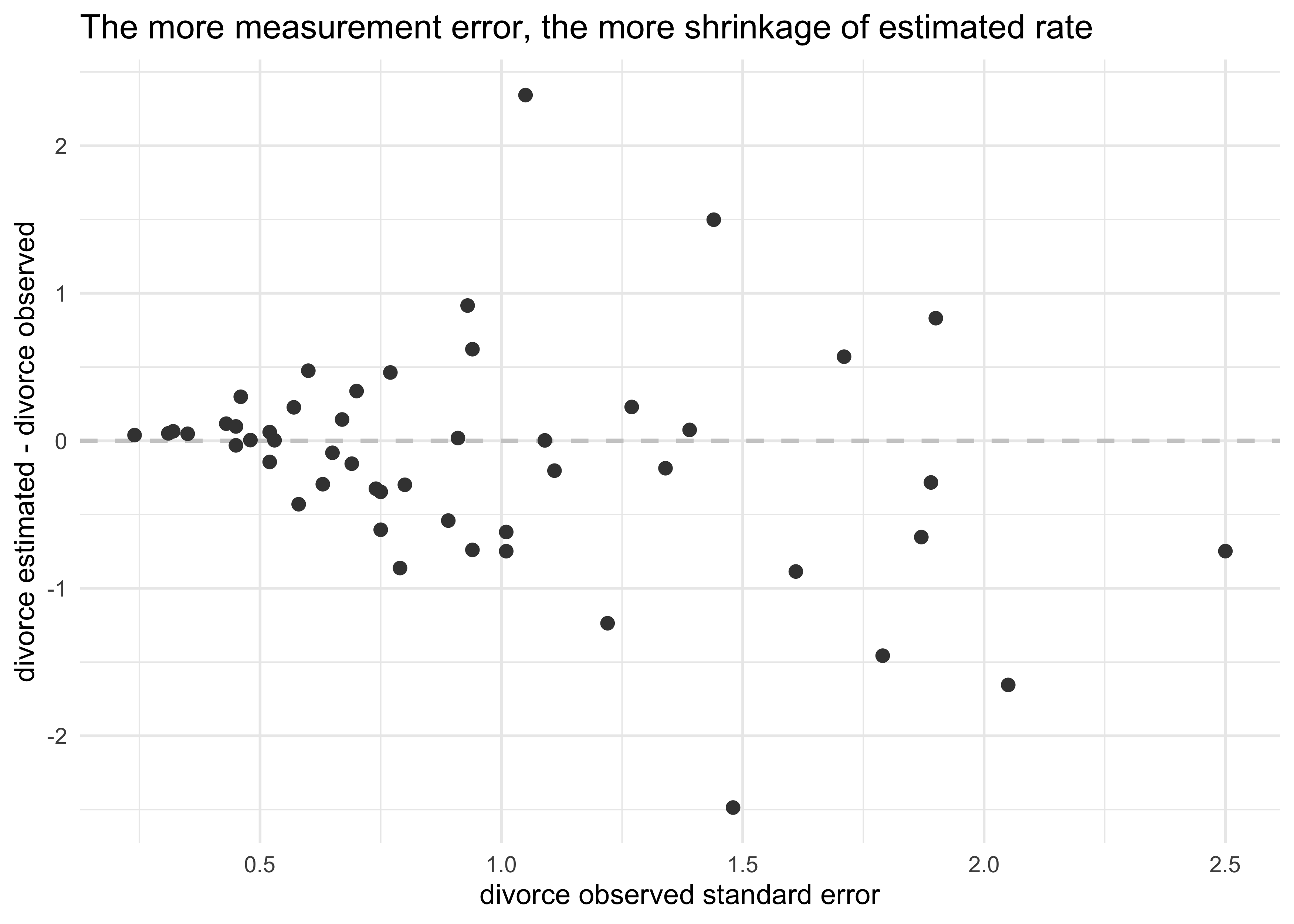
- can see why because states with very high or low ages at marriage tended to have high uncertainty in divorce rates
- in the model, the rates with greater uncertainty have been
shrunk towards the mean that is more defined by the measurements
with smaller measurement error
- this is shrinkage
estimated_divorce_post <- extract.samples(m14_1)$div_est

d %>%
    mutate(estimated_divorce = apply(estimated_divorce_post, 2, mean)) %>%
    ggplot(aes(x = divorce_se, y = estimated_divorce - divorce)) +
    geom_hline(yintercept = 0, lty = 2, color = light_grey, size = 0.8) +
    geom_point(size = 2, color = dark_grey) +
    labs(x = "divorce observed standard error",
         y = "divorce estimated - divorce observed",
         title = "The more measurement error, the more shrinkage of estimated rate")
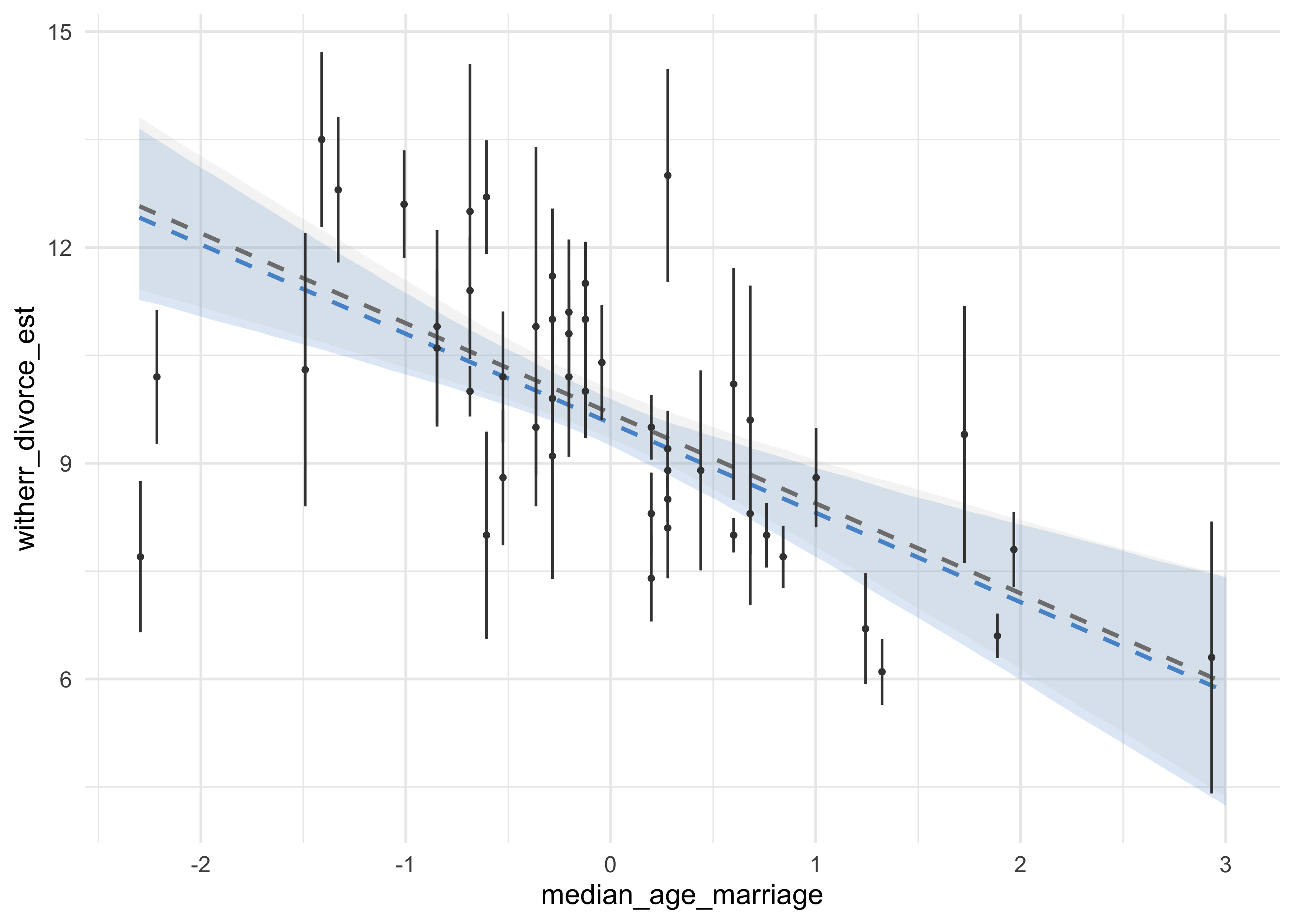
- below, the model without accounting for measurement error is created and the posterior estimates of median age are shown
stash("m14_1_noerr", depends_on = "dlist", {
    m14_1_noerr <- map2stan(
        alist(
            div_obs ~ dnorm(mu, sigma),
            mu <- a + bA*A + bR*R,
            a ~ dnorm(0, 10),
            bA ~ dnorm(0, 10),
            bR ~ dnorm(0, 10),
            sigma ~ dcauchy(0, 10)
        ),
        data = dlist,
        WAIC = FALSE,
        iter = 5e3, warmup = 1e3, chains = 2, cores = 2,
        control = list(adapt_delta = 0.95)
    )
})
#> Loading stashed object.
median_age_seq <- seq(-2.3, 3, length.out = 100)
avg_marriage <- mean(dlist$R)
pred_d <- tibble(A = median_age_seq, R = avg_marriage)
m14_1_post <- link(m14_1, data = pred_d)
#> [ 100 / 1000 ][ 200 / 1000 ][ 300 / 1000 ][ 400 / 1000 ][ 500 / 1000 ][ 600 / 1000 ][ 700 / 1000 ][ 800 / 1000 ][ 900 / 1000 ][ 1000 / 1000 ]
m14_1_noerr_post <- link(m14_1_noerr, data = pred_d)
#> [ 100 / 1000 ][ 200 / 1000 ][ 300 / 1000 ][ 400 / 1000 ][ 500 / 1000 ][ 600 / 1000 ][ 700 / 1000 ][ 800 / 1000 ][ 900 / 1000 ][ 1000 / 1000 ]
pred_d_post <- pred_d %>%
    rename(median_age_marriage = A, marriage = R) %>%
    mutate(witherr_divorce_est = apply(m14_1_post, 2, mean),
           noerr_divorce_est = apply(m14_1_noerr_post, 2, mean)) %>%
    bind_cols(
        apply(m14_1_post, 2, PI) %>%
            pi_to_df() %>%
            set_names(c("with_err_5", "with_err_94")),
        apply(m14_1_noerr_post, 2, PI) %>%
            pi_to_df() %>%
            set_names(c("no_err_5", "no_err_94"))
    )

d %>%
    mutate(median_age_marriage = scale_nums(median_age_marriage)) %>%
    ggplot(aes(x = median_age_marriage)) +
    geom_ribbon(aes(ymin = with_err_5, ymax = with_err_94),
                data = pred_d_post,
                alpha = 0.2, fill = blue) +
    geom_ribbon(aes(ymin = no_err_5, ymax = no_err_94),
                data = pred_d_post,
                alpha = 0.2, fill = light_grey) +
    geom_line(aes(y = witherr_divorce_est),
              data = pred_d_post,
              color = blue, lty = 2, size = 0.8) +
    geom_line(aes(y = noerr_divorce_est),
              data = pred_d_post,
              color = grey, lty = 2, size = 0.8) +
    geom_linerange(aes(ymin = divorce - divorce_se, ymax = divorce + divorce_se),
                   size = 0.5, color = dark_grey) +
    geom_point(aes(y = divorce), size = 0.7, color = dark_grey)
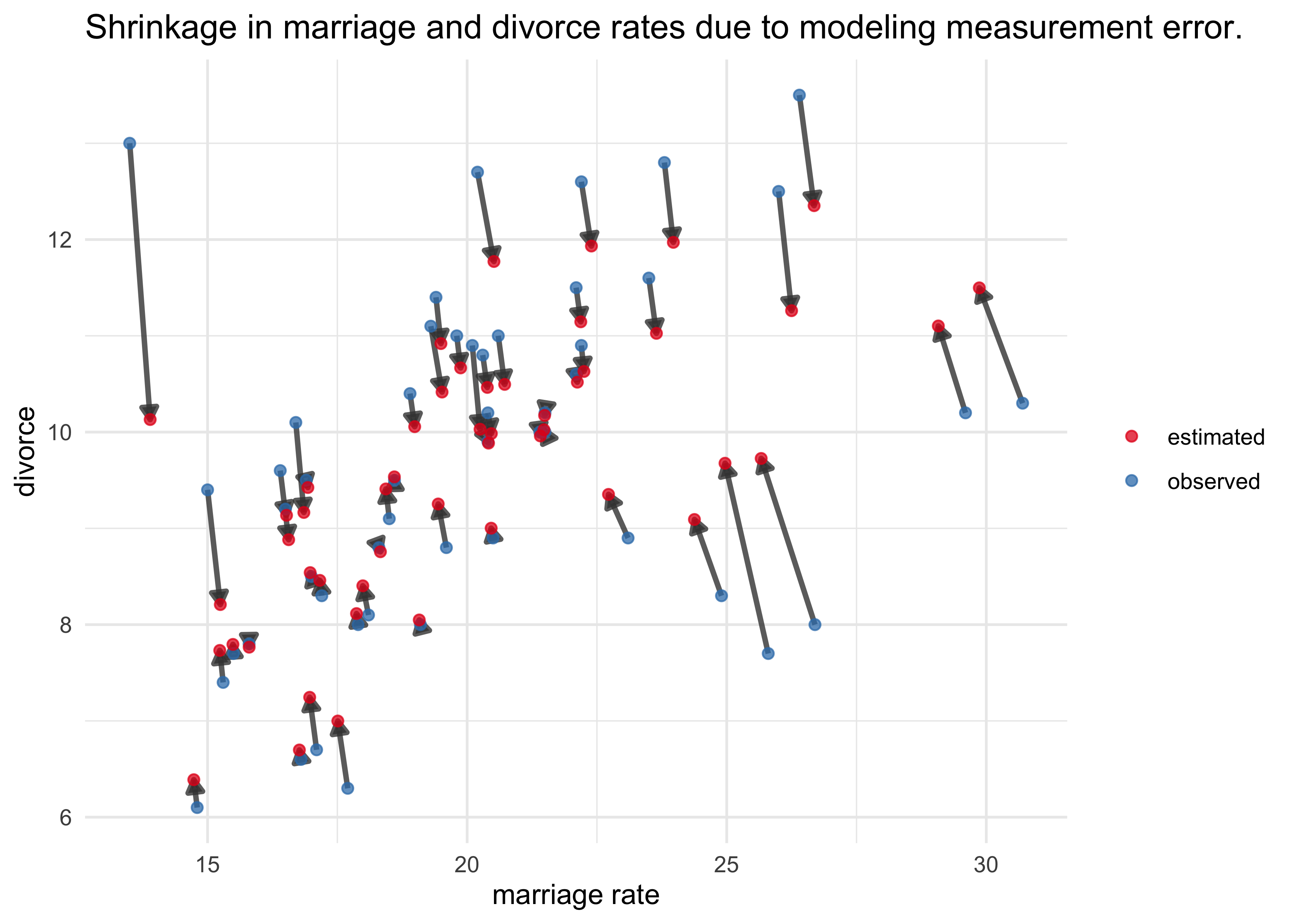
14.1.2 Error on both outcome and predictor
- measurement error on predictors and outcome
- think about the problem generatively:
- each observed predictor value is a draw from a distribution with an unknown mean and standard deviation
- we can define a vector of parameters, one per unknown, and make them the means of a Gaussian distributions
- think about the problem generatively:
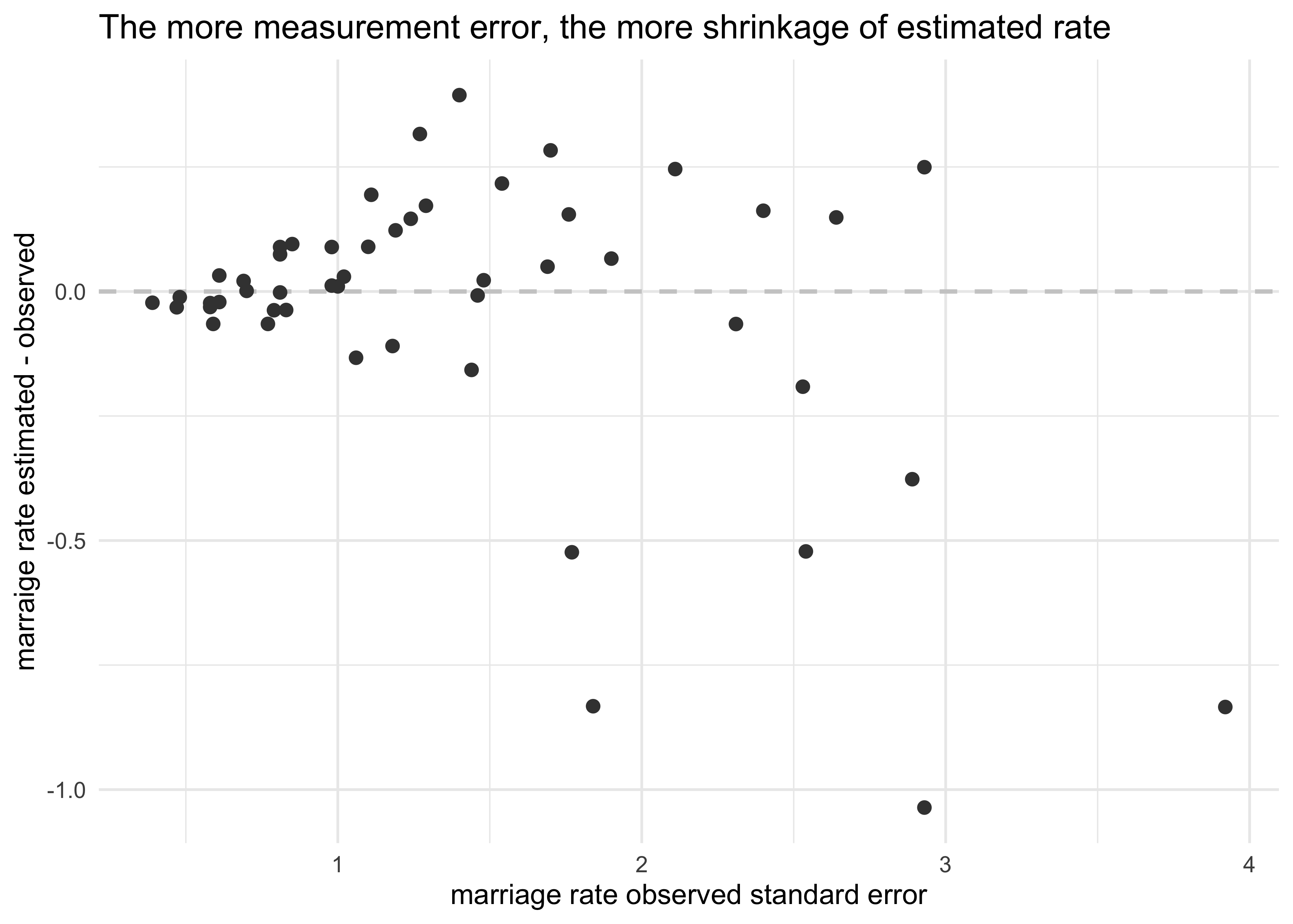
- example in the divorce data with error on marriage rate
$$ D_{\text{est}, i} \sim \text{Normal}(\mu_i, \sigma) $$ $$ \mu_i = \alpha + \beta_A A_i + \beta_R R_{\text{est}, i} $$ $$ D_{\text{obs}, i} \sim \text{Normal}(D_{\text{est}, i}, D_{\text{SE}, i}) $$ $$ R_{\text{obs}, i} \sim \text{Normal}(R_{\text{est}, i}, R_{\text{SE}, i}) $$ $$ \alpha \sim \text{Normal}(0, 10) $$ $$ \beta_A \sim \text{Normal}(0, 10) $$ $$ \beta_R \sim \text{Normal}(0, 10) $$ $$ \sigma \sim \text{Cauchy}(0, 2.5) $$
dlist <- d %>%
    select(div_obs = divorce, div_sd = divorce_se,
           mar_obs = marriage, mar_sd = marriage_se,
           A = median_age_marriage)

stash("m14_2", depends_on = "dlist", {
    m14_2 <- map2stan(
        alist(
            div_est ~ dnorm(mu, sigma),
            mu <- a + bA*A + bR*mar_est[i],
            div_obs ~ dnorm(div_est, div_sd),
            mar_obs ~ dnorm(mar_est, mar_sd),
            a ~ dnorm(0, 10),
            bA ~ dnorm(0, 10),
            bR ~ dnorm(0, 10),
            sigma ~ dcauchy(0, 2.5)
        ),
        data = dlist,
        start = list(div_est = dlist$div_obs,
                     mar_est = dlist$mar_obs),
        WAIC = FALSE,
        iter = 5e3, warmup = 1e3, chains = 3, cores = 3,
        control = list(adapt_delta = 0.95)
    )
})
#> Loading stashed object.
precis(m14_2)
#> 100 vector or matrix parameters hidden. Use depth=2 to show them.

#>             mean         sd         5.5%      94.5%    n_eff    Rhat4
#> a     20.8720987 6.82182042  9.666433007 31.5786222 2891.271 1.000815
#> bA    -0.5400344 0.21819074 -0.882554474 -0.1794355 3217.269 1.000645
#> bR     0.1384014 0.08306949  0.009533411  0.2730756 2740.129 1.000991
#> sigma  1.0975441 0.20658634  0.787150660  1.4454654 2899.495 1.000417
estimated_marriage_post <- extract.samples(m14_2)$mar_est

d %>%
    mutate(est_marriage = apply(estimated_marriage_post, 2, mean)) %>%
    ggplot(aes(x = marriage_se, y = est_marriage - marriage)) +
    geom_hline(yintercept = 0, lty = 2, color = light_grey, size = 0.8) +
    geom_point(size = 2, color = dark_grey) +
    labs(x = "marriage rate observed standard error",
         y = "marraige rate estimated - observed",
         title = "The more measurement error, the more shrinkage of estimated rate")
m14_2_post_samples <- extract.samples(m14_2)

d_est <- tibble(loc = d$loc) %>%
    mutate(divorce = apply(m14_2_post_samples$div_est, 2, mean),
           marriage = apply(m14_2_post_samples$mar_est, 2, mean),
           obs_est = "estimated")

d %>%
    select(loc, divorce, marriage) %>%
    add_column(obs_est = "observed") %>%
    bind_rows(d_est) %>%
    ggplot(aes(marriage, divorce)) +
    geom_path(aes(group = loc), alpha = 0.8, size = 1, color = dark_grey,
              arrow = arrow(length = unit(2, "mm"), ends = "last", type = "closed")) +
    geom_point(aes(color = obs_est), size = 1.7, alpha = 0.75) +
    scale_color_brewer(palette = "Set1") +
    labs(x = "marriage rate",
         y = "divorce",
         title = "Shrinkage in marriage and divorce rates due to modeling measurement error.",
         color = NULL)
14.2 Missing data
14.2.1 Imputing neocortex
- example using Bayesian imputation to impute the missing
neocortex.percvalues in themilkdata- use information from other columns
- the imputed values will have posterior distributions (better than a point estimate)
- Missing Completely At Random (MCAR): an imputation model that assumes the points that are missing are missing due to random chance
- simultaneously model the predictor variable that has missing value
and the outcome variable
- the present values will produce estimates that comprise a prior for each missing value
- then use these priors for estimating the relationship between the predictor and outcome
- think of the predictor with missing data as a mixture of data and parameters
- below is the formula for the model
- the $N_i \sim \text{Normal}(v, \sigma_N)$ is the distribution
for the neocortex percent values
- if $N_i$ is observed, then it is a likelihood
- if $N_i$ is missing, then it is a prior distribution
- the $N_i \sim \text{Normal}(v, \sigma_N)$ is the distribution
for the neocortex percent values
$$ k_i \sim \text{Normal}(\mu_i, \sigma) $$ $$ \mu_i = \alpha + \beta_N N_i + \beta_M \log M_i $$ $$ N_i \sim \text{Normal}(\nu, \sigma_N) $$ $$ \alpha \sim \text{Normal}(0, 100) $$ $$ \beta_N \sim \text{Normal}(0, 10) $$ $$ \beta_M \sim \text{Normal}(0, 10) $$ $$ \sigma \sim \text{Normal}(0, 1) $$ $$ \nu \sim \text{Normal}(0.5, 1) $$ $$ \sigma_N \sim \text{Cauchy}(0, 1) $$
- several ways to implement this model
# Load the data.
data("milk")
d <- as_tibble(milk) %>%
    janitor::clean_names() %>%
    mutate(neocortex_prop = neocortex_perc / 100,
           logmass = log(mass))

data_list <- d %>%
    select(kcal = kcal_per_g,
           neocortex = neocortex_prop,
           logmass)

stash("m14_3", depends_on = "data_list", {
    m14_3 <- map2stan(
        alist(
            kcal ~ dnorm(mu, sigma),
            mu <- a + bN*neocortex + bM*logmass,
            neocortex ~ dnorm(nu, sigma_N),
            a  ~ dnorm(0, 100),
            c(bN, bM) ~ dnorm(0, 10),
            nu ~ dnorm(0.5, 1),
            sigma_N ~ dcauchy(0, 1),
            sigma ~ dcauchy(0, 1)
        ),
        data = data_list, iter = 1e4, chains = 2, cores = 2
    )
})
#> Loading stashed object.
precis(m14_3, depth = 2)
#>                             mean         sd       5.5%       94.5%     n_eff
#> neocortex_impute[1]   0.63198252 0.05026444  0.5539061  0.71393638  7375.298
#> neocortex_impute[2]   0.62439457 0.05082310  0.5451610  0.70625252  7744.599
#> neocortex_impute[3]   0.62249738 0.05117690  0.5430334  0.70445442  6915.737
#> neocortex_impute[4]   0.65219955 0.04870903  0.5753615  0.73034213  9502.564
#> neocortex_impute[5]   0.70097228 0.04849636  0.6242957  0.78068875  8857.497
#> neocortex_impute[6]   0.65650853 0.05003216  0.5794043  0.73647672  8697.525
#> neocortex_impute[7]   0.68701466 0.04796190  0.6106304  0.76329911 10188.181
#> neocortex_impute[8]   0.69656253 0.04807550  0.6195392  0.77177427  8898.820
#> neocortex_impute[9]   0.71240683 0.04935848  0.6328875  0.78997705  9123.654
#> neocortex_impute[10]  0.64580225 0.04967418  0.5672966  0.72321254  8802.068
#> neocortex_impute[11]  0.65796422 0.04869620  0.5816114  0.73455664  9168.917
#> neocortex_impute[12]  0.69548363 0.04997620  0.6147117  0.77310037  8148.645
#> a                    -0.53192286 0.47208501 -1.2685262  0.23265819  2414.370
#> bN                    1.89757591 0.73606344  0.7053816  3.05058129  2343.718
#> bM                   -0.06920106 0.02248688 -0.1051405 -0.03326359  2847.262
#> nu                    0.67132733 0.01378503  0.6496262  0.69302024  7428.522
#>                          Rhat4
#> neocortex_impute[1]  0.9998108
#> neocortex_impute[2]  1.0004621
#> neocortex_impute[3]  0.9999360
#> neocortex_impute[4]  0.9999356
#> neocortex_impute[5]  0.9998307
#> neocortex_impute[6]  0.9999942
#> neocortex_impute[7]  1.0000914
#> neocortex_impute[8]  1.0002591
#> neocortex_impute[9]  0.9998138
#> neocortex_impute[10] 0.9998282
#> neocortex_impute[11] 0.9999832
#> neocortex_impute[12] 0.9998682
#> a                    1.0002426
#> bN                   1.0003011
#> bM                   1.0005604
#> nu                   0.9998143
#>  [ reached 'max' / getOption("max.print") -- omitted 2 rows ]
- for comparison, also build a model with the missing data dropped
dcc <- d[complete.cases(d$neocortex_prop), ]
data_list_cc <- dcc %>%
    select(kcal = kcal_per_g, neocortex = neocortex_prop, logmass)

stash("m14_3_cc", depends_on = "data_list_cc", {
    m14_3_cc <- map2stan(
        alist(
            kcal ~ dnorm(mu, sigma),
            mu <- a + bN*neocortex + bM*logmass,
            a ~ dnorm(0, 100),
            c(bN, bM) ~ dnorm(0, 10),
            sigma ~ dcauchy(0, 1)
        ),
        data = data_list_cc, iter = 1e4, chains = 2, cores = 2
    )
})
#> Loading stashed object.
precis(m14_3_cc)
#>             mean         sd       5.5%       94.5%    n_eff    Rhat4
#> a     -1.0774335 0.57905288 -1.9994215 -0.17402779 2435.072 1.000556
#> bN     2.7813725 0.90188209  1.3639509  4.22172504 2414.102 1.000478
#> bM    -0.0962560 0.02811227 -0.1401678 -0.05196683 2992.969 1.000027
#> sigma  0.1385882 0.02948439  0.1000234  0.19141166 3061.492 1.000285
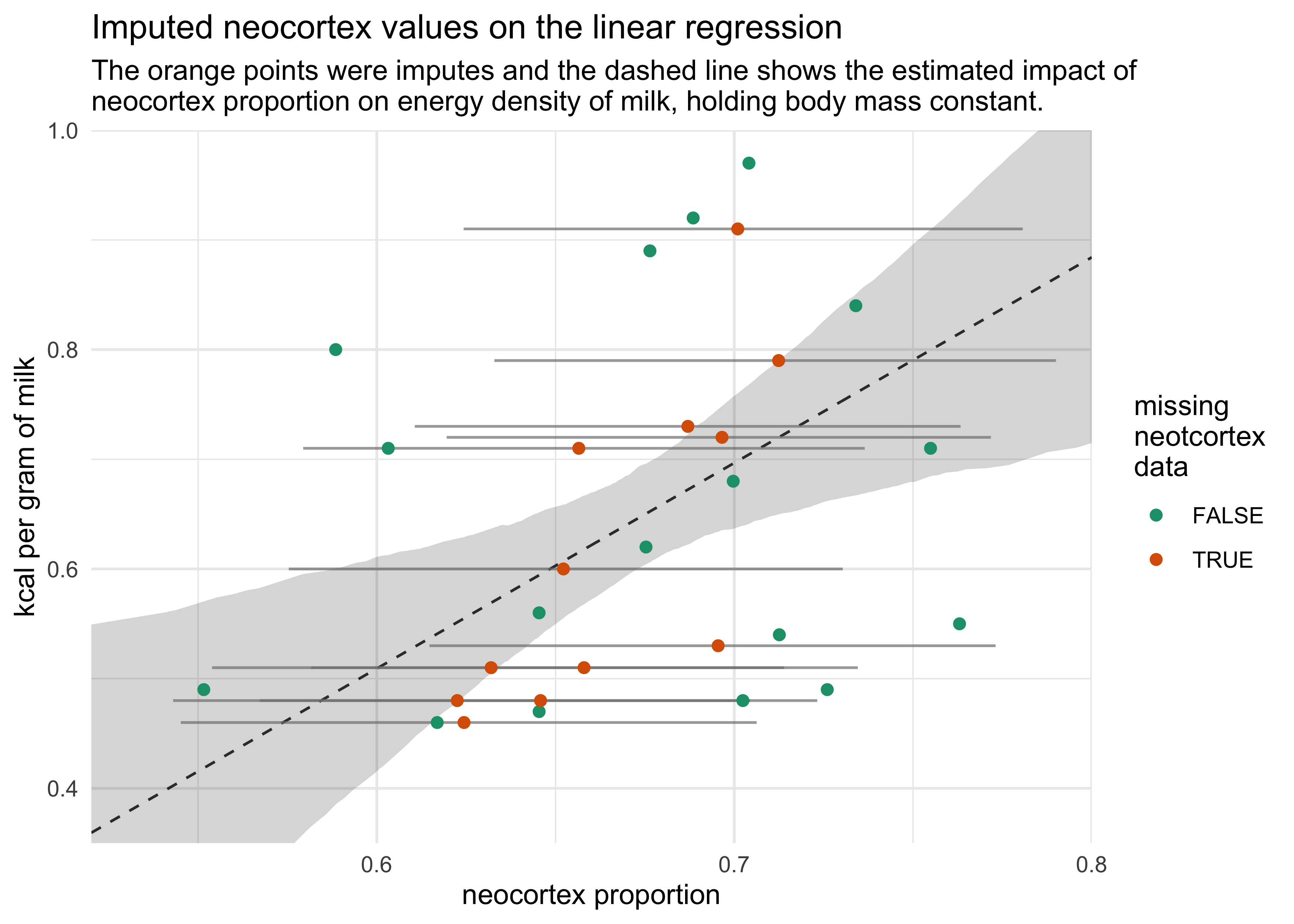
- including the incomplete cases moves the posterior mean for neocortext proportion from 2.8 to 1.9 and for body mass from -0.1 to -0.07
- the following plot shows the imputed data comparing the neocortex proportion to the kcal per gram of milk
m14_3_post <- extract.samples(m14_3)

neocortex_seq <- seq(0.45, 0.8, length.out = 500)
logmass_avg <- mean(d$logmass)
m14_3_pred_d <- tibble(neocortex = neocortex_seq, logmass = logmass_avg)
m14_3_pred <- link(m14_3, data = m14_3_pred_d)
#> [ 100 / 1000 ][ 200 / 1000 ][ 300 / 1000 ][ 400 / 1000 ][ 500 / 1000 ][ 600 / 1000 ][ 700 / 1000 ][ 800 / 1000 ][ 900 / 1000 ][ 1000 / 1000 ]
m14_3_pred_d %<>%
    mutate(kcal_est = apply(m14_3_pred, 2, mean)) %>%
    bind_cols(apply(m14_3_pred, 2, PI) %>% pi_to_df()) %>%
    filter(neocortex > 0.52) %>%
    mutate(x5_percent = scales::squish(x5_percent, range = c(0.35, 1.0)),
           x94_percent = scales::squish(x94_percent, range = c(0.35, 1.0)))

imputed_neocortex_prop <- tibble(
    neocortex_prop_est = apply(m14_3_post$neocortex_impute, 2, mean)
) %>%
    bind_cols(apply(m14_3_post$neocortex_impute, 2, PI) %>% pi_to_df()) %>%
    mutate(miss_num_idx = row_number())

d %>%
    mutate(missing_neocortex = is.na(neocortex_prop)) %>%
    group_by(missing_neocortex) %>%
    mutate(miss_num_idx = row_number()) %>%
    ungroup() %>%
    mutate(miss_num_idx = ifelse(missing_neocortex, miss_num_idx, NA)) %>%
    left_join(imputed_neocortex_prop, by = "miss_num_idx") %>%
    mutate(neocortex_prop = ifelse(missing_neocortex, neocortex_prop_est, neocortex_prop)) %>%
    ggplot(aes(neocortex_prop)) +
    geom_ribbon(aes(x = neocortex, ymin = x5_percent, ymax = x94_percent),
                data = m14_3_pred_d,
                alpha = 0.2) +
    geom_line(aes(x = neocortex, y = kcal_est),
              data = m14_3_pred_d,
              alpha = 0.8, lty = 2) +
    geom_linerange(aes(y = kcal_per_g, xmin = x5_percent, xmax = x94_percent),
                   alpha = 0.7, color = grey) +
    geom_point(aes(y = kcal_per_g, color = missing_neocortex),
               size = 1.7) +
    scale_color_brewer(palette = "Dark2") +
    scale_x_continuous(expand = c(0, 0)) +
    scale_y_continuous(limits = c(0.35, 1.0), expand = c(0, 0)) +
    labs(x = "neocortex proportion",
         y = "kcal per gram of milk",
         title = "Imputed neocortex values on the linear regression",
         subtitle = "The orange points were imputes and the dashed line shows the estimated impact of\nneocortex proportion on energy density of milk, holding body mass constant.",
         color = "missing\nneotcortex\ndata")
#> Warning: Removed 17 rows containing missing values (geom_segment).
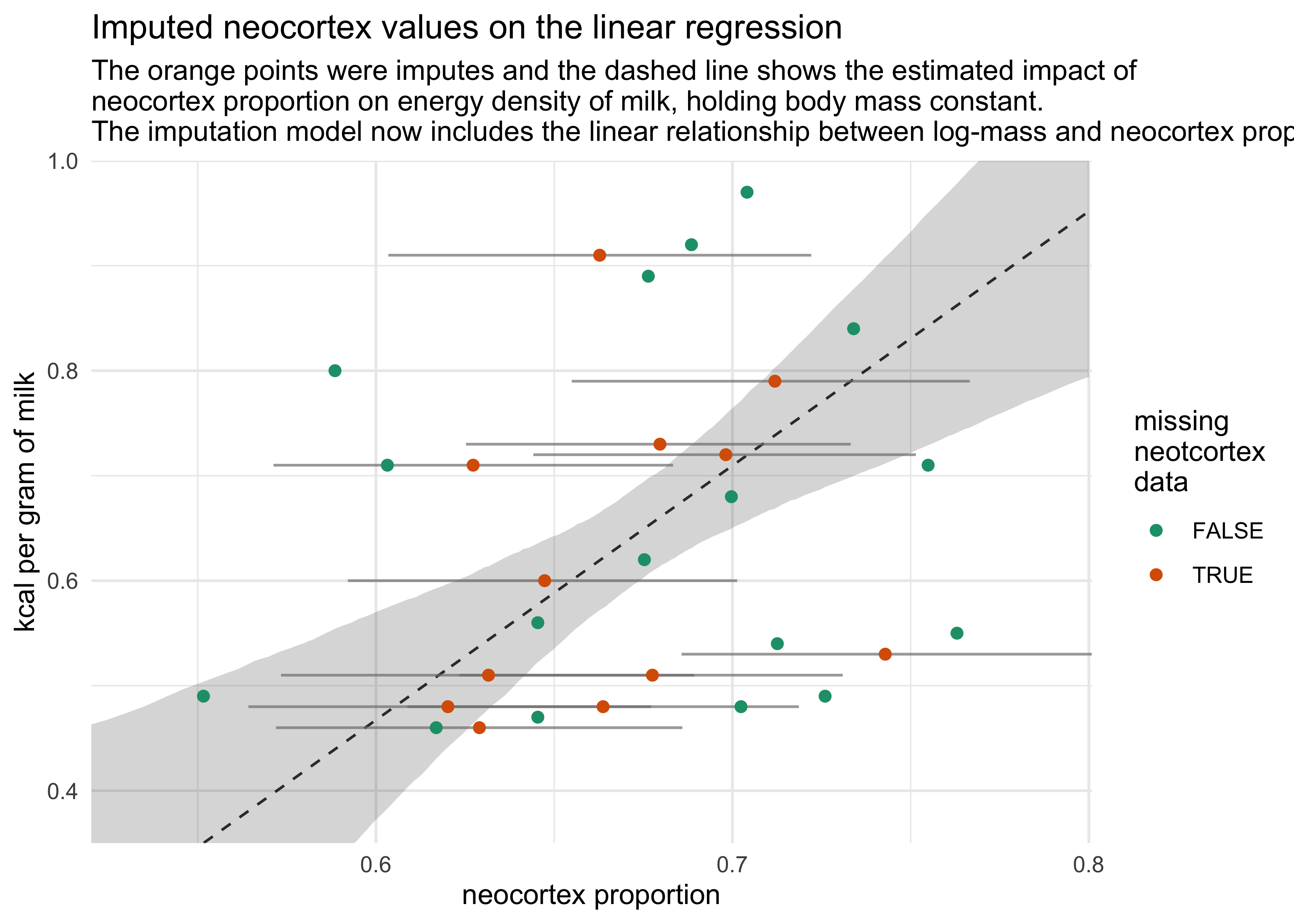
14.2.2 Improving the imputation model
- improve the imputation model by accounting for the associations
among the predictors themselves
- make the following change to the model in place of $N_i \sim \text{Normal}(\nu, \sigma_N)$
- describe a linear relationship between the neocortex and log mass using $\alpha_N$ and $\gamma_M$
$$ N_i \sim \text{Normal}(\nu_i, \sigma_N) $$ $$ \nu = \alpha_N + \gamma_M \log M_i $$
stash("m14_4", depends_on = "data_list", {
    m14_4 <- map2stan(
        alist(
            kcal ~ dnorm(mu, sigma),
            mu <- a + bN*neocortex + bM*logmass,
            neocortex ~ dnorm(nu, sigma_N),
            nu <- a_N + gM*logmass,
            a  ~ dnorm(0, 100),
            a_N ~ dnorm(0.5, 1),
            c(bN, bM, gM) ~ dnorm(0, 10),
            sigma_N ~ dcauchy(0, 1),
            sigma ~ dcauchy(0, 1)
        ),
        data = data_list, iter = 1e4, chains = 2, cores = 2
    )
})
#> Loading stashed object.
precis(m14_4, depth = 2)
#>                             mean         sd       5.5%       94.5%    n_eff
#> neocortex_impute[1]   0.63156684 0.03637137  0.5733482  0.68927381 7393.707
#> neocortex_impute[2]   0.62901603 0.03594894  0.5719131  0.68595036 7020.294
#> neocortex_impute[3]   0.62017155 0.03581074  0.5642132  0.67718484 7479.422
#> neocortex_impute[4]   0.64732183 0.03463234  0.5921108  0.70133376 9219.062
#> neocortex_impute[5]   0.66276294 0.03704484  0.6034764  0.72211903 7277.220
#> neocortex_impute[6]   0.62725276 0.03531693  0.5712322  0.68333750 8092.599
#> neocortex_impute[7]   0.67966994 0.03409030  0.6252496  0.73318426 9503.017
#> neocortex_impute[8]   0.69813729 0.03391513  0.6441340  0.75147620 8922.176
#> neocortex_impute[9]   0.71191533 0.03501537  0.6549321  0.76659425 8487.077
#> neocortex_impute[10]  0.66371400 0.03461562  0.6087791  0.71863769 8378.396
#> neocortex_impute[11]  0.67755183 0.03409107  0.6233687  0.73095538 9481.087
#> neocortex_impute[12]  0.74287971 0.03589815  0.6857309  0.80081662 8040.294
#> a                    -0.85248132 0.48314860 -1.6012869 -0.07478841 2768.100
#> a_N                   0.63821972 0.01244794  0.6181859  0.65775742 4877.374
#> bN                    2.41331628 0.75582831  1.1939338  3.58663403 2728.551
#> bM                   -0.08780227 0.02315191 -0.1240904 -0.05057892 3544.639
#>                          Rhat4
#> neocortex_impute[1]  1.0007608
#> neocortex_impute[2]  1.0002637
#> neocortex_impute[3]  0.9998614
#> neocortex_impute[4]  0.9998810
#> neocortex_impute[5]  1.0002131
#> neocortex_impute[6]  1.0000067
#> neocortex_impute[7]  0.9998735
#> neocortex_impute[8]  0.9999079
#> neocortex_impute[9]  0.9998110
#> neocortex_impute[10] 1.0001477
#> neocortex_impute[11] 0.9998439
#> neocortex_impute[12] 1.0000570
#> a                    1.0001689
#> a_N                  1.0001027
#> bN                   1.0001993
#> bM                   1.0004306
#>  [ reached 'max' / getOption("max.print") -- omitted 3 rows ]
m14_4_post <- extract.samples(m14_4)

neocortex_seq <- seq(0.45, 0.8, length.out = 500)
logmass_avg <- mean(d$logmass)
m14_4_pred_d <- tibble(neocortex = neocortex_seq, logmass = logmass_avg)
m14_4_pred <- link(m14_4, data = m14_4_pred_d)
#> [ 100 / 1000 ][ 200 / 1000 ][ 300 / 1000 ][ 400 / 1000 ][ 500 / 1000 ][ 600 / 1000 ][ 700 / 1000 ][ 800 / 1000 ][ 900 / 1000 ][ 1000 / 1000 ]
m14_4_pred_d %<>%
    mutate(kcal_est = apply(m14_4_pred$mu, 2, mean)) %>%
    bind_cols(apply(m14_4_pred$mu, 2, PI) %>% pi_to_df()) %>%
    filter(neocortex > 0.52) %>%
    mutate(x5_percent = scales::squish(x5_percent, range = c(0.35, 1.0)),
           x94_percent = scales::squish(x94_percent, range = c(0.35, 1.0)))

imputed_neocortex_prop <- tibble(
    neocortex_prop_est = apply(m14_4_post$neocortex_impute, 2, mean)
) %>%
    bind_cols(apply(m14_4_post$neocortex_impute, 2, PI) %>% pi_to_df()) %>%
    mutate(miss_num_idx = row_number())

d %>%
    mutate(missing_neocortex = is.na(neocortex_prop)) %>%
    group_by(missing_neocortex) %>%
    mutate(miss_num_idx = row_number()) %>%
    ungroup() %>%
    mutate(miss_num_idx = ifelse(missing_neocortex, miss_num_idx, NA)) %>%
    left_join(imputed_neocortex_prop, by = "miss_num_idx") %>%
    mutate(neocortex_prop = ifelse(missing_neocortex, neocortex_prop_est, neocortex_prop)) %>%
    ggplot(aes(neocortex_prop)) +
    geom_ribbon(aes(x = neocortex, ymin = x5_percent, ymax = x94_percent),
                data = m14_4_pred_d,
                alpha = 0.2) +
    geom_line(aes(x = neocortex, y = kcal_est),
              data = m14_4_pred_d,
              alpha = 0.8, lty = 2) +
    geom_linerange(aes(y = kcal_per_g, xmin = x5_percent, xmax = x94_percent),
                   alpha = 0.7, color = grey) +
    geom_point(aes(y = kcal_per_g, color = missing_neocortex),
               size = 1.7) +
    scale_color_brewer(palette = "Dark2") +
    scale_x_continuous(expand = c(0, 0)) +
    scale_y_continuous(limits = c(0.35, 1.0), expand = c(0, 0)) +
    labs(x = "neocortex proportion",
         y = "kcal per gram of milk",
         title = "Imputed neocortex values on the linear regression",
         subtitle = "The orange points were imputes and the dashed line shows the estimated impact of\nneocortex proportion on energy density of milk, holding body mass constant.\nThe imputation model now includes the linear relationship between log-mass and neocortex prop.",
         color = "missing\nneotcortex\ndata")
#> Warning: Removed 45 row(s) containing missing values (geom_path).

#> Warning: Removed 17 rows containing missing values (geom_segment).
Joshua Cook
Graduate Student
My research interests include cancer genetics and evolution. I also learning about programming and computer science in general.