Chapter 13. Adventures In Covariance

• this chapter will show how to specify varying slopes in combination with varying intercepts
  • enables pooling to improve estimates of how different units respond to or are influenced by predictor variables
  • also improves the estimates of intercepts by “borrowing information across parameter types”
  • “varying slope models are massive interaction machines”

13.1 Varying slopes by construction

• pool information across intercepts and slopes by modeling the joint population of intercepts and slopes
  • modeling their covariance
  • assigning a 2D Gaussian distribution to both the intercepts (first dimension) and the slopes (second dimension)
• the variance-covariance matrix for a fit model describes how each parameters posterior probability is associated with one another
  • varying intercepts have variation, varying slopes have variation, and intercepts and slopes covary
• use example of visiting coffee shops:
  • visit different cafes, order a coffee, and record the wait time
    • previously, used varying intercepts, one for each cafe
  • also record the time of day
    • the average wait time is longer in the mornings than afternoons because they are busier in the mornings
  • different cafes vary in their average wait times and their differences between morning and afternoon
    • the differences in wait time by time of day are the slopes
  • cafes covary in their intercepts and slopes
    • because the popular cafes have much longer wait times in the morning leading to large differences between morning and afternoon

$$ \mu_i = \alpha_{\text{cafe}[i]} + \beta_{\text{cafe}[i]} A_i $$

13.1.1 Simulate the population

• define the population of cafes
  • define the average wait time in the morning and afternoon
  • define the correlation between them

a <- 3.5        # average morning wait time
b <- -1         # average difference afternoon wait time
sigma_a <- 1    # standard deviation in intercepts
sigma_b <- 0.5  # standard deviation in slopes
rho <- -0.7     # correlation between intercepts and slopes

• use these values to simulate a sample of cafes
  • define the multivariate Gaussian with a vector of means and a 2x2 matrix of variances and covariances

Mu <- c(a, b)  # vector of two means

• the matrix of variances and covariances is arranged as follows

$$ \begin{pmatrix} \sigma_\alpha^2 & \sigma_\alpha \sigma_\beta \rho $$ $$ \sigma_\alpha \sigma_\beta \rho & \sigma_\beta^2 \end{pmatrix} $$

• can construct the matrix explicitly

cov_ab <- sigma_a * sigma_b * rho
Sigma <- matrix(c(sigma_a^2, cov_ab, cov_ab, sigma_b^2), nrow = 2)
Sigma

#>       [,1]  [,2]
#> [1,]  1.00 -0.35
#> [2,] -0.35  0.25

• another way to build the variance-covariance matrix using matrix multiplication
  • this is likely a better approach with larger models

sigmas <- c(sigma_a, sigma_b)
Rho <- matrix(c(1, rho, rho, 1), nrow = 2)
Sigma <- diag(sigmas) %*% Rho %*% diag(sigmas)
Sigma

#>       [,1]  [,2]
#> [1,]  1.00 -0.35
#> [2,] -0.35  0.25

• now can simulate 20 cafes, each with their own intercept and slope

N_cafes <- 20

• simulate from a multivariate Gaussian using mvnorm() from the ‘MASS’ package
  • returns a matrix of $\text{cafe} \times (\text{intercept}, \text{slope})$

library(MASS)

set.seed(5)
vary_effects <- mvrnorm(n = N_cafes, mu = Mu, Sigma = Sigma)
head(vary_effects)

#>          [,1]       [,2]
#> [1,] 4.223962 -1.6093565
#> [2,] 2.010498 -0.7517704
#> [3,] 4.565811 -1.9482646
#> [4,] 3.343635 -1.1926539
#> [5,] 1.700971 -0.5855618
#> [6,] 4.134373 -1.1444539

# Split into separate vectors for ease of use later.
a_cafe <- vary_effects[, 1]
b_cafe <- vary_effects[, 2]
cor(a_cafe, b_cafe)

#> [1] -0.5721537

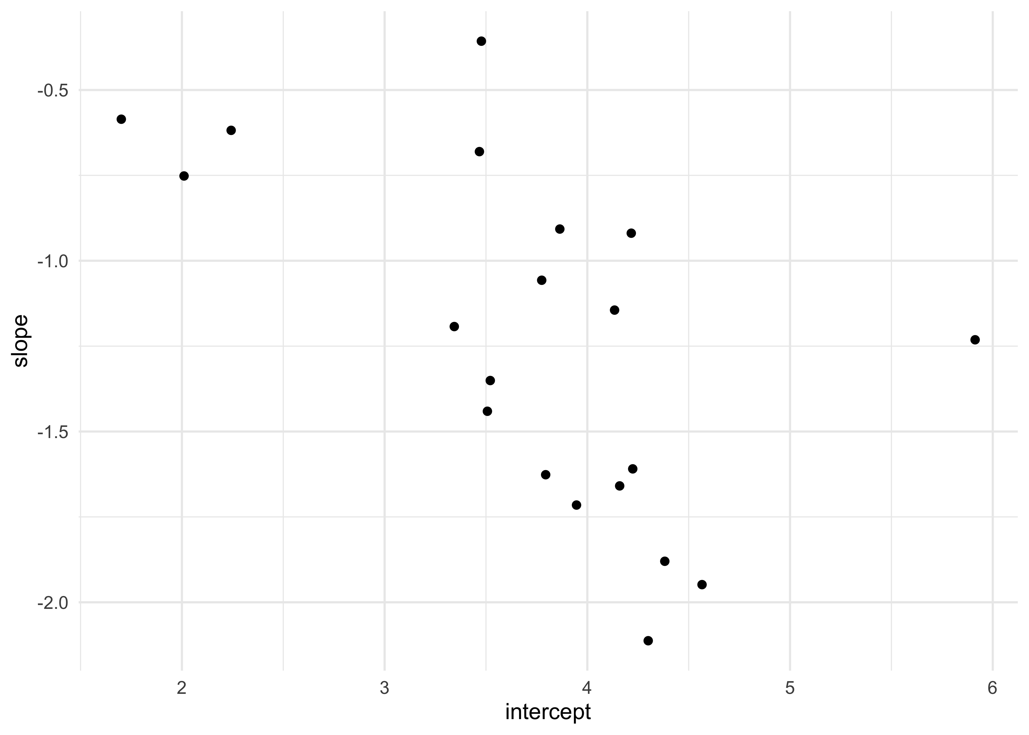
• plot of the varying effects

as.data.frame(vary_effects) %>%
    as_tibble() %>%
    set_names(c("intercept", "slope")) %>%
    ggplot(aes(x = intercept, y = slope)) +
    geom_point()

13.1.2 Simulate observations

• simulate the visits to each cafe
  • 10 visits to each cafe, 5 in the morning and 5 in the afternoon

N_visits <- 10
afternoon <- rep(0:1, N_visits * N_cafes / 2)
cafe_id <- rep(1:N_cafes, each = N_visits)

# Get the average wait time for each cafe in the morning and afternoon.
mu <- a_cafe[cafe_id] + b_cafe[cafe_id] * afternoon

sigma <- 0.5  # Standard deviation within cafes

# Sample wait times with each cafes unique average wait time per time of day.
wait_times <- rnorm(N_visits*N_cafes, mu, sigma)

d <- tibble(cafe = cafe_id, afternoon, wait = wait_times)
d

#> # A tibble: 200 x 3
#>     cafe afternoon  wait
#>    <int>     <int> <dbl>
#>  1     1         0  5.00
#>  2     1         1  2.21
#>  3     1         0  4.19
#>  4     1         1  3.56
#>  5     1         0  4.00
#>  6     1         1  2.90
#>  7     1         0  3.78
#>  8     1         1  2.38
#>  9     1         0  3.86
#> 10     1         1  2.58
#> # … with 190 more rows

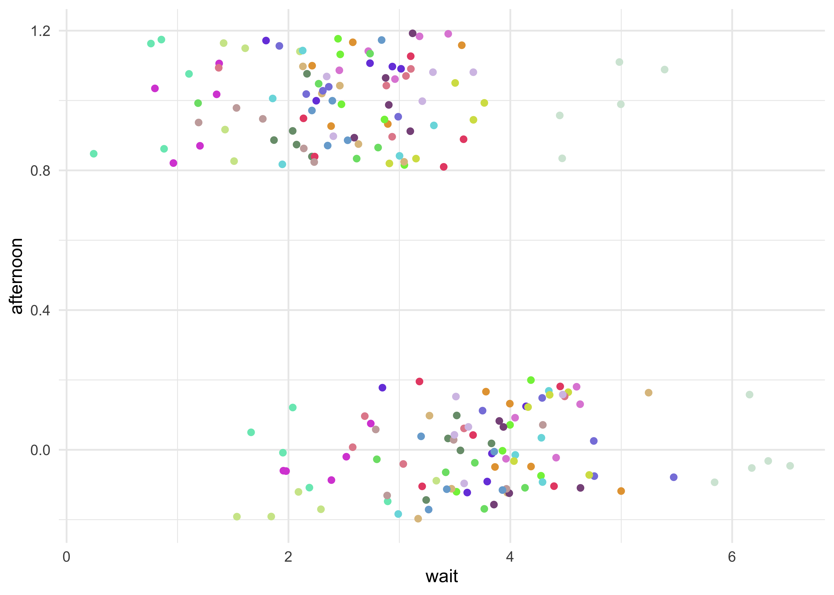
d %>%
    ggplot(aes(x = wait, y = afternoon, color = factor(cafe))) +
    geom_jitter(width = 0, height = 0.2) +
    scale_color_manual(values = randomcoloR::distinctColorPalette(N_cafes),
                       guide = FALSE)

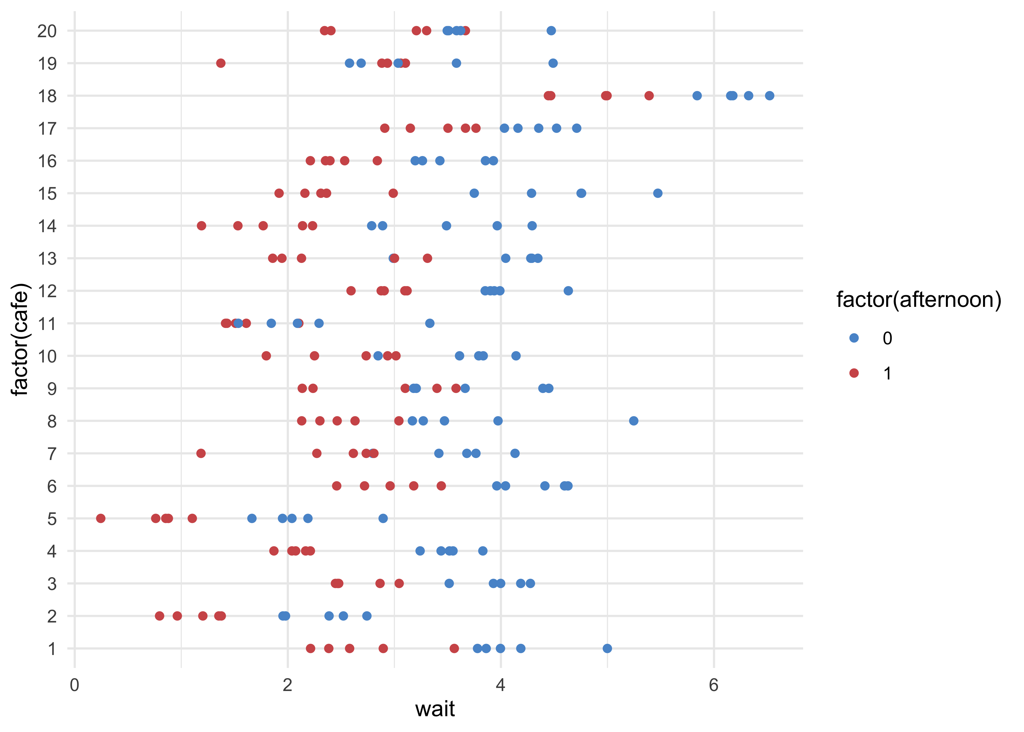
d %>%
    ggplot(aes(x = wait, y = factor(cafe), color = factor(afternoon))) +
    geom_point() +
    scale_color_manual(values = c(blue, red))

13.1.3 The varying slopes model

• model with varying intercepts and slopes (explanation follows)

$$ W_i (_i, ) $$ $$

*i = *{$$i$$} + _{$$i$$} A_i $$ $$

(

, ) $$ $$

=

$$ $$

(0,10) $$ $$ (0,10) \ (0, 1) \ *(0, 1) \ *(0, 1) \ (2) $$

• the third like defines the population of varying intercepts and slopes
  • each cafe has an intercept and slope with a prior distribution defined by the 2D Gaussian distribution with means $\alpha$ and $\beta$ and covariance matrix $\text{S}$

$$ \begin{bmatrix} \alpha_\text{cafe} $$ $$ \beta_\text{cafe} \end{bmatrix} \sim \text{MVNormal}( \begin{bmatrix} \alpha $$ $$ \beta \end{bmatrix}, \textbf{S} ) $$

• the next line defines the variance-covariance matrix $\textbf{S}$
  • factoring it into simple standard deviations $\sigma_\alpha$ and $\sigma_\beta$ and a correlation matrix $\textbf{R}$
  • there are other ways to do this, but this formulation helps understand the inferred structure of the varying effects

$$ \textbf{S} = \begin{pmatrix} \sigma_\alpha & 0 $$ $$ 0 &\sigma_\beta \end{pmatrix} \textbf{R} \begin{pmatrix} \sigma_\alpha & 0 $$ $$ 0 &\sigma_\beta \end{pmatrix} $$

• the correlation matrix has a prior defined as $\textbf{R} \sim \text{LKJcorr}(2)$
  • the correlation matrix will have the structure: $\begin{pmatrix} 1 & \rho $$ $$ \rho & 1 \end{pmatrix}$ where $\rho$ is the correlation between the intercepts and slopes
  • with additional varying slopes, there are more correlation parameters, but the $\text{LKJcorr}$ prior will still work
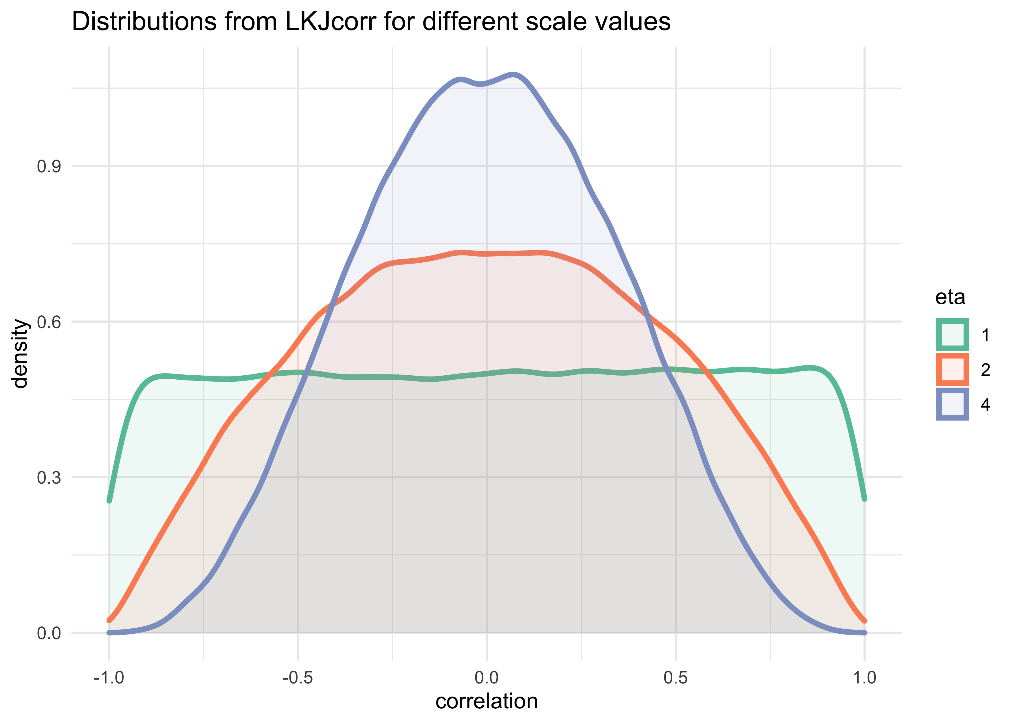
  • the $\text{LKJcorr}(2)$ prior defines a weakly informative prior on $\rho$ that is skeptical of extreme correlations near -1 and 1
  • it has a single parameter $\eta$ that controls how “skeptical” the prior is of large correlations
    • if $\eta=1$, the prior is flat from -1 to 1
    • a large value of $\eta$ the mass of the distribution moves towards 0

tibble(eta = c(1, 2, 4)) %>%
    mutate(value = map(eta, ~ rlkjcorr(1e5, K = 2, eta = .x)[, 1, 2])) %>%
    unnest(value) %>%
    ggplot(aes(x = value)) +
    geom_density(aes(color = factor(eta), fill = factor(eta)), 
                 size = 1.3, alpha = 0.1) +
    scale_color_brewer(palette = "Set2") +
    scale_fill_brewer(palette = "Set2") +
    labs(x = "correlation",
         y = "density",
         title = "Distributions from LKJcorr for different scale values",
         color = "eta", fill = "eta")

• now can fit the model

stash("m13_1", {
    m13_1 <- map2stan(
        alist(
            wait ~ dnorm(mu, sigma),
            mu <- a_cafe[cafe] + b_cafe[cafe]*afternoon,
            c(a_cafe, b_cafe)[cafe] ~ dmvnorm2(c(a, b), sigma_cafe, Rho),
            a ~ dnorm(0, 10),
            b ~ dnorm(0, 10),
            sigma_cafe ~ dcauchy(0, 2),
            sigma ~ dcauchy(0, 2),
            Rho ~ dlkjcorr(2)
        ),
        data = d,
        iter = 5e3, warmup = 2e3, chains = 2
    )
})

#> Loading stashed object.

precis(m13_1, depth = 1)

#> 46 vector or matrix parameters hidden. Use depth=2 to show them.

#>             mean         sd      5.5%      94.5%    n_eff     Rhat4
#> a      3.7411232 0.22805989  3.386143  4.1040327 6673.815 0.9998308
#> b     -1.2443621 0.13662408 -1.458389 -1.0304374 5965.979 0.9999912
#> sigma  0.4648216 0.02624559  0.424598  0.5085003 6410.601 0.9999077

• inspection of the posterior distribution of varying effects
  • start with the posterior correlation between intercepts and slopes
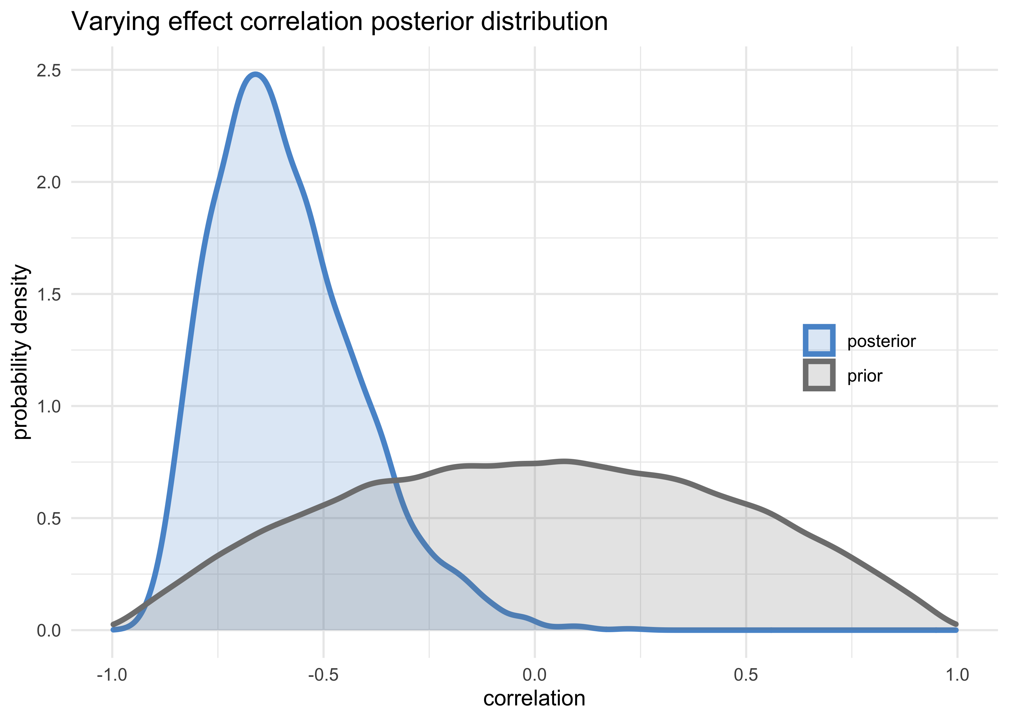
    • the posterior distribution of the correlation between varying effects is decidedly negative

post <- extract.samples(m13_1)

tribble(
    ~name, ~value,
    "posterior", post$Rho[, 1, 2],
    "prior", rlkjcorr(1e5, K = 2, eta = 2)[, 1, 2]
) %>%
    unnest(value) %>%
    ggplot(aes(x = value, color = name, fill = name)) +
    geom_density(size = 1.3, alpha = 0.2) +
    scale_color_manual(values = c(blue, grey)) +
    scale_fill_manual(values = c(blue, grey)) +
    theme(legend.title = element_blank(),
          legend.position = c(0.85, 0.5)) +
    labs(x = "correlation",
         y = "probability density",
         title = "Varying effect correlation posterior distribution")

• consider the shrinkage
  • the inferred correlation between varying effects pooled information across them
  • and the inferred variation within each varying effect was pooled
  • together the variances and correlation define a multivariate Gaussian prior for the varying effects
  • this prior regularizes the intercepts and slopes
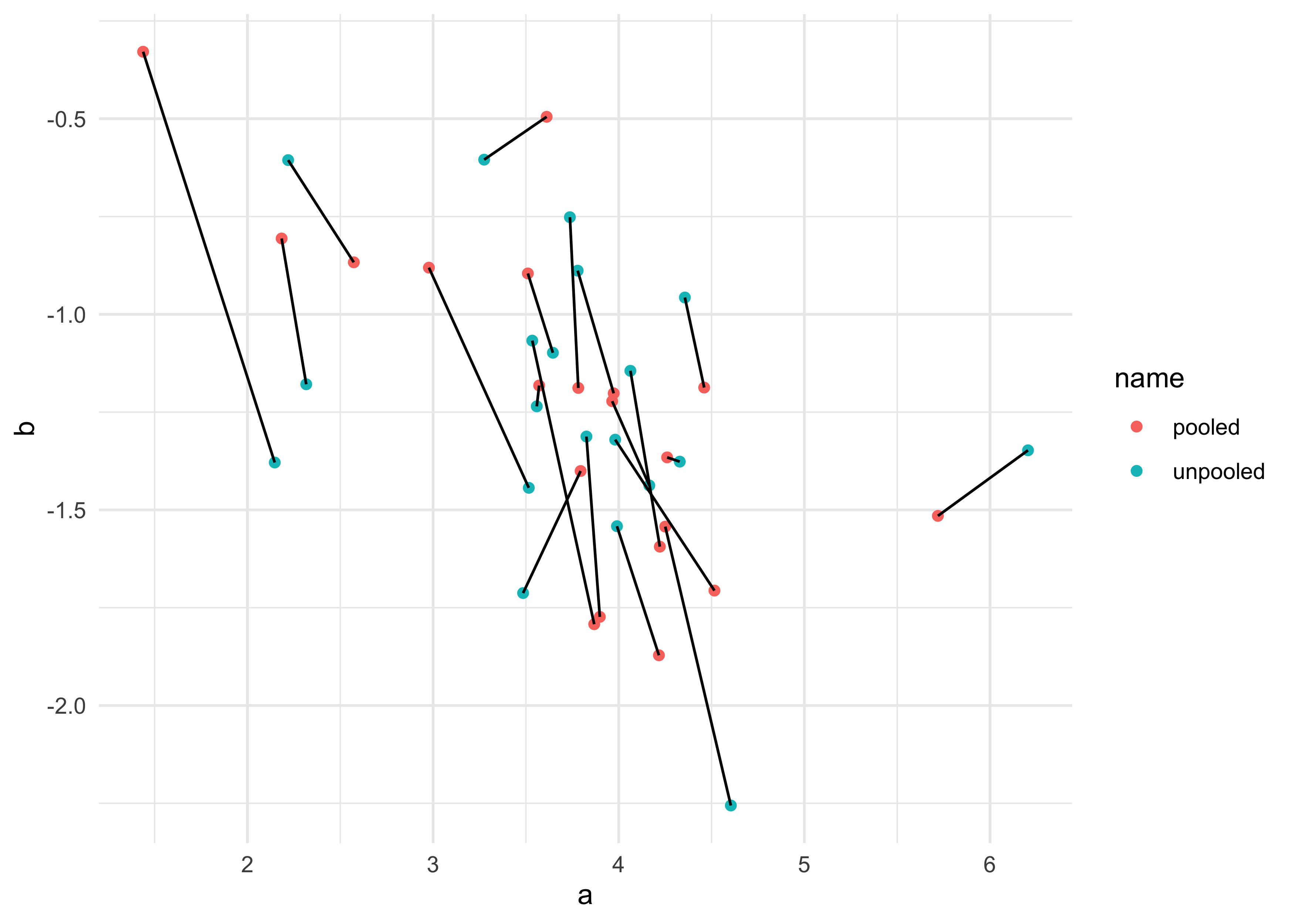
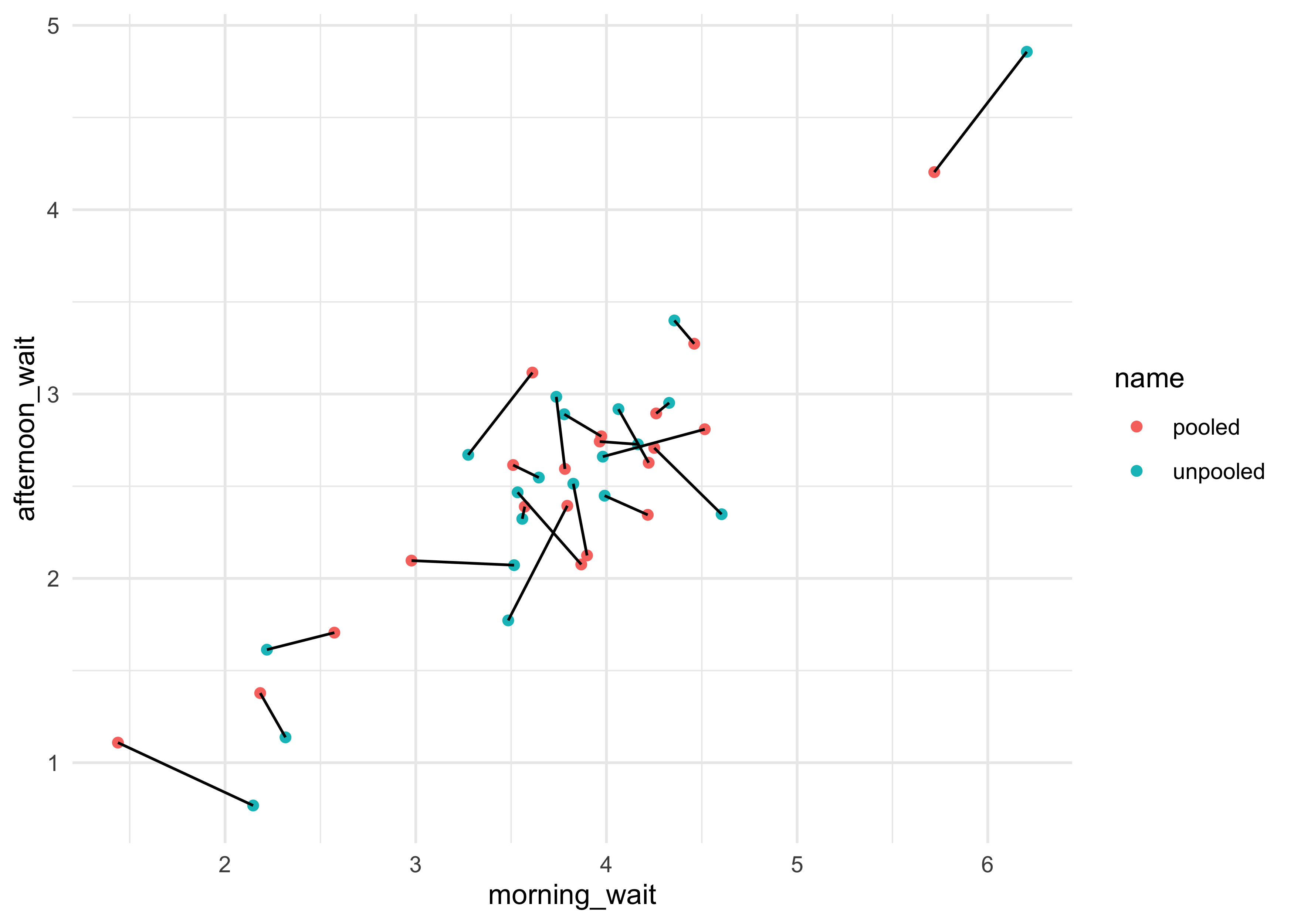
• plot the posterior mean varying effects
  • compare them to the raw, unpooled estimates
  • also plot the inferred prior for the population of intercepts and slopes

There is something wrong with the following 2 plots, but I cannot figure out what went wrong.

# Raw, unpooled estimates for alpha and beta.
a1 <- map_dbl(1:N_cafes, function(i) {
    mean(d$wait[d$cafe == i & d$afternoon == 0])
})

b1 <- map_dbl(1:N_cafes, function(i) {
    mean(d$wait[d$cafe == i & d$afternoon == 1])
})
b1 <- b1 - a1

# Extract posterior means of partially pooled estimates.
post <- extract.samples(m13_1)
a2 <- apply(post$a_cafe, 2, mean)
b2 <- apply(post$b_cafe, 2, mean)

tribble(
    ~ name, ~ a, ~ b,
    "unpooled", a1, b1,
    "pooled", a2, b2
) %>%
    unnest(c(a, b)) %>%
    group_by(name) %>%
    mutate(cafe = row_number()) %>%
    ungroup() %>%
    ggplot(aes(x = a, y = b)) +
    geom_point(aes(color = name)) +
    geom_line(aes(group = cafe))

• can do the same for the estimated wait times for each cafe in the morning and afternoon

tribble(
    ~ name, ~ morning_wait, ~ afternoon_wait,
    "unpooled", a1, a1 + b1,
    "pooled", a2, a2 + b2
) %>%
    unnest(c(morning_wait, afternoon_wait)) %>%
    group_by(name) %>%
    mutate(cafe = row_number()) %>%
    ungroup() %>%
    ggplot(aes(x = morning_wait, y = afternoon_wait)) +
    geom_point(aes(color = name)) +
    geom_line(aes(group = cafe))

13.2 Example: Admission decisions and gender

• return to the admissions data and use varying slopes
  • help appreciate how variation in slopes arises
  • and how correlation between intercepts and slopes can provide insight into the underlying process
• from previous models of the UCBadmit data:
  • important to have varying means across department otherwise, get wrong inference about gender
  • did not account for variation in how departments treat male and female applications

data("UCBadmit")
d <- as_tibble(UCBadmit) %>%
    janitor::clean_names() %>%
    mutate(male = as.numeric(applicant_gender == "male"),
           dept_id = coerce_index(dept))

13.2.1 Varying intercepts

• first model with only the varying intercepts

$$ A_i \sim \text{Binomial}(n_i, p_i) $$ $$ \text{logit}(p_i) = \alpha_{\text{dept}[i]} + \beta m_i $$ $$ \alpha_\text{dept} \sim \text{Normal}(\alpha, \sigma) $$ $$ \alpha \sim \text{Normal}(0, 10) $$ $$ \beta \sim \text{Normal}(0, 1) $$ $$ \sigma \sim \text{HalfCauchy}(0, 2) $$ $$ $$

stash("m13_2", {
    m13_2 <- map2stan(
        alist(
            admit ~ dbinom(applications, p),
            logit(p) <- a_dept[dept_id] + bm*male,
            a_dept[dept_id] ~ dnorm(a, sigma_dept),
            a ~ dnorm(0, 10),
            bm ~ dnorm(0, 1),
            sigma_dept ~ dcauchy(0, 2)
        ),
        data = d,
        warmup = 500, iter = 4500, chains = 3
    )
})

#> Loading stashed object.

precis(m13_2, depth = 2)

#>                   mean         sd       5.5%       94.5%     n_eff     Rhat4
#> a_dept[1]   0.67633553 0.09912824  0.5172706  0.83647836  7434.742 0.9998820
#> a_dept[2]   0.62865617 0.11487786  0.4462060  0.81244427  7451.327 0.9999420
#> a_dept[3]  -0.58407578 0.07381761 -0.7037524 -0.46666875  9691.393 1.0000113
#> a_dept[4]  -0.61607540 0.08473505 -0.7513828 -0.47998152  8592.307 0.9998870
#> a_dept[5]  -1.05883405 0.09832475 -1.2173306 -0.90286742 12118.564 0.9999736
#> a_dept[6]  -2.60914320 0.15654731 -2.8607355 -2.36390139 10442.752 1.0000161
#> a          -0.61042302 0.67864636 -1.6337291  0.40209932  5772.182 1.0004375
#> bm         -0.09471168 0.08101324 -0.2257535  0.03522607  5929.314 1.0000314
#> sigma_dept  1.49095940 0.58217912  0.8576455  2.52329901  5681.029 1.0003271

• interpretation
  • effect of male is similar that found in Chapter 10 (“Counting and Classification”)
    • the intercept is effectively uninteresting, if perhaps slightly negative
  • because we included the global mean $\alpha$ in the prior for the varying intercepts, the a_dept[i] values are all deviations from a

13.2.2 Varying effects of being male

• now we can consider the variation in gender bias among departments
  • use varying slopes
• the data is imbalanced
  • the sample sizes vary a lot across departments
  • pooling will have a stronger effect for cases with fewer applicants

$$ A_i (n_i, p_i) $$ $$ (p_i) = *{$$i$$} + *{$$i$$} m_i \

(

, ) $$ $$

(0, 10) $$ $$ (0, 1) \

=

$$ $$

(*, *) (0, 2) $$ $$ (2) $$

stash("m13_3", {
    m13_3 <- map2stan(
        alist(
            admit ~ dbinom(applications, p),
            logit(p) <- a_dept[dept_id] + bm_dept[dept_id]*male,
            c(a_dept, bm_dept)[dept_id] ~ dmvnorm2(c(a, bm), sigma_dept, Rho),
            a ~ dnorm(0, 10),
            bm ~ dnorm(0, 1),
            sigma_dept ~ dcauchy(0, 2),
            Rho ~ dlkjcorr(2)
        ),
        data = d,
        warmup = 1e3, iter = 5e3, chains = 4
    )
})

#> Loading stashed object.

precis(m13_3, depth = 2)

#> 4 matrix parameters hidden. Use depth=3 to show them.

#>                      mean         sd       5.5%      94.5%     n_eff     Rhat4
#> bm_dept[1]    -0.79410911 0.26621581 -1.2314113 -0.3769640  7777.776 1.0001133
#> bm_dept[2]    -0.21452957 0.32827223 -0.7442305  0.2976597  7706.047 1.0002087
#> bm_dept[3]     0.08210299 0.13916525 -0.1436567  0.3047949 14294.571 1.0001411
#> bm_dept[4]    -0.09107295 0.14166835 -0.3189406  0.1369298 12245.517 1.0003159
#> bm_dept[5]     0.12616695 0.18522579 -0.1659927  0.4251783 13979.943 0.9998708
#> bm_dept[6]    -0.12371601 0.26875987 -0.5601516  0.3021377 11343.429 1.0000722
#> a_dept[1]      1.30684485 0.25312427  0.9145892  1.7201724  7768.113 1.0000828
#> a_dept[2]      0.74419573 0.32704100  0.2349881  1.2721056  7974.643 1.0001940
#> a_dept[3]     -0.64703547 0.08559338 -0.7820730 -0.5101126 15352.790 1.0001005
#> a_dept[4]     -0.61945023 0.10575932 -0.7888304 -0.4512668 12336.691 1.0001413
#> a_dept[5]     -1.13473049 0.11377576 -1.3178663 -0.9556382 14357.673 0.9999653
#> a_dept[6]     -2.60003282 0.19884720 -2.9234768 -2.2882146 13404.431 1.0000262
#> a             -0.50152540 0.73756490 -1.6147961  0.6207689  8686.590 1.0001169
#> bm            -0.16333123 0.23571418 -0.5286623  0.1998200  8991.565 1.0000629
#> sigma_dept[1]  1.68379712 0.65077176  0.9809923  2.7911987  7190.902 1.0000942
#> sigma_dept[2]  0.50115741 0.25052608  0.2116896  0.9321738  7771.766 1.0003994

• focus on what the addition of varying slopes has revealed
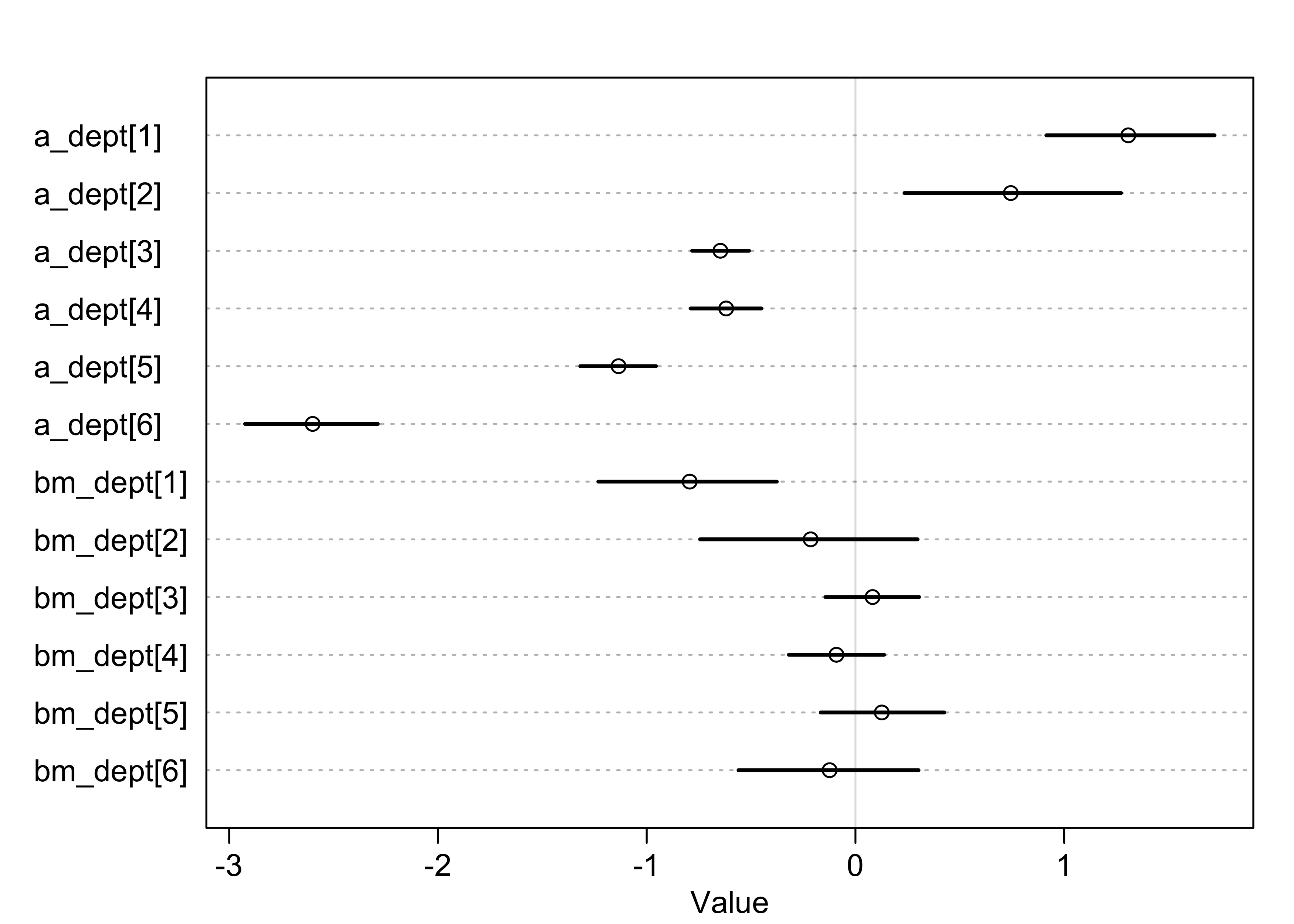
  • plot below shows marginal posterior distributions for the varying effects
  • the intercepts are quite varied, but the slopes are all quite close to 0
    • suggests that the departments had different rates of admissions, but none discriminated between male and females
    • one standout is the slope for department 1 which suggests some bias against females
      • department 1 also has the largest intercept, so look into the correlation between slopes and intercepts next

plot(precis(m13_3, pars = c("a_dept", "bm_dept"), depth = 2))

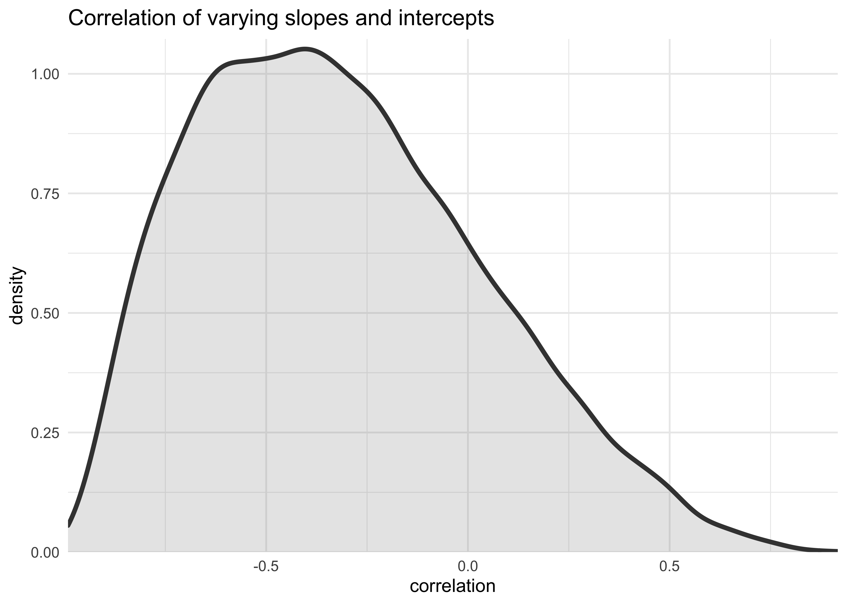
13.2.3 Shrinkage

• following plot shows the posterior distribution for the correlation between slope and intercept
  • negative correlation: the higher the admissions rate, the lower the slope

post <- extract.samples(m13_3)
tibble(posterior_rho = post$Rho[, 1, 2]) %>%
    ggplot(aes(x = posterior_rho)) +
    geom_density(size = 1.3, color = dark_grey, fill = grey, alpha = 0.2) +
    scale_x_continuous(expand = expansion(mult = c(0, 0))) +
    scale_y_continuous(expand = expansion(mult = c(0, 0.02))) +
    labs(x = "correlation",
         y = "density",
         title = "Correlation of varying slopes and intercepts")

13.2.4 Model comparison

• also fit a model that ignores gender for purposes of comparison

stash("m13_4", {
    m13_4 <- map2stan(
        alist(
            admit ~ dbinom(applications, p),
            logit(p) <- a_dept[dept_id],
            a_dept[dept_id] ~ dnorm(a, sigma_dept),
            a ~ dnorm(0, 10),
            sigma_dept ~ dcauchy(0, 2)
        ),
        data = d,
        warmup = 500, iter = 4500, chains = 3
    )
})

#> Loading stashed object.

compare(m13_2, m13_3, m13_4)

#>           WAIC       SE    dWAIC      dSE     pWAIC      weight
#> m13_3 5190.940 57.26937  0.00000       NA 11.094350 0.987737123
#> m13_4 5200.945 56.84874 10.00469 6.820917  5.939283 0.006639735
#> m13_2 5201.277 56.93248 10.33705 6.516639  6.864329 0.005623142

• interpretation:
  • the model with no slope for differences in gender m13_4 performs the same out-of-sample performance as the model with a single slope for a constant effect of gender m13_2
  • the model with varying slopes suggests that even though the slope is near zero, it is worth modeling as a separate distribution

13.3 Example: Cross-classified chimpanzees with varying slopes

• use chimpanzee data to model multiple varying intercepts and/or slopes
  • varying intercepts for actor and block
  • varying slopes for prosocial option and the interaction between prosocial and the presence of another chimpanzee
• non-centered parameterization (see later for explanation and example)
  • there are always several ways to formulate a model that are mathematically equivalent
  • however, they can result in different sampling results, so the parameterization is part of the model
• cross-classified varying slopes model
  • use multiple linear models to compartmentalize sub-models for the intercepts and each slope
  • $\mathcal{A}i$, $\mathcal{B}{P,i}$, and $\mathcal{B}_{PC,i}$ are the sub-models

$$ L_i \sim \text{Binomial}(1, p_i) $$ $$ \text{logit}(p_i) = \mathcal{A}i + (\mathcal{B}{p,i} + \mathcal{B}{PC,i} C_i) P_i $$ $$ \mathcal{A}i = \alpha + \alpha{\text{actor}[i]} + \alpha{\text{block}[i]} $$ $$ \mathcal{B}{P,i} = \beta_P + \beta{P,\text{actor}[i]} + \beta_{P,\text{block}[i]} $$ $$ \mathcal{B}_{PC,i} = \beta_P + \beta_{PC,\text{actor}[i]} + \beta_{PC,\text{block}[i]} $$ $$ $$

• below is the formulation for the multivariate priors
  • one multivariate Gaussian per cluster of the data (actor and block)
  • for this model, each is 3D, one for each variable in the model
    • this can be adjusted to have different varying effects in different cluster types
  • these priors state that the actors and blocks come from different statistical populations
    • within each, three features for each actor or block are related through a covariance matrix for the population ($\textbf{S}$)
    • the mean for each prior is 0 because there is an average value in the linear models already ($\alpha$, $\beta_P$, and $\beta_{PC,i}$)

$$

$$ $$

$$

data("chimpanzees")
d <- as_tibble(chimpanzees) %>%
    select(-recipient) %>%
    rename(block_id = block)

stash("m13_6", {
    m13_6 <- map2stan(
        alist(
            pulled_left ~ dbinom(1, p),
            logit(p) <- A + (BP + BPC*condition) * prosoc_left,
            A <- a + a_actor[actor] + a_block[block_id],
            BP <- bp + bp_actor[actor] + bp_block[block_id],
            BPC <- bpc + bpc_actor[actor] + bpc_block[block_id],
            
            c(a_actor, bp_actor, bpc_actor)[actor] ~ dmvnorm2(0, sigma_actor, Rho_actor),
            c(a_block, bp_block, bpc_block)[block_id] ~ dmvnorm2(0, sigma_block, Rho_block),
            
            c(a, bp, bpc) ~ dnorm(0, 1),
            sigma_actor ~ dcauchy(0, 2),
            sigma_block ~ dcauchy(0, 2),
            Rho_actor ~ dlkjcorr(4),
            Rho_block ~ dlkjcorr(4)
        ),
        data = d,
        iter = 5e3, warmup = 1e3, chains = 3
    )
})

#> Loading stashed object.

precis(m13_6, depth = 1)

#> 63 vector or matrix parameters hidden. Use depth=2 to show them.

#>            mean        sd        5.5%     94.5%    n_eff    Rhat4
#> a    0.23573453 0.6666099 -0.90821904 1.2611100  934.458 1.001440
#> bp   0.70892674 0.4052890  0.05423901 1.3312395 3817.263 1.000350
#> bpc -0.03931986 0.4317621 -0.68617116 0.6610651 2216.997 1.001548

• there was an issue with the HMC sampling
  • can often just do more sampling to get over it, but other times the chains may not converge
  • this is where non-centered parameterization can help

In map2stan(alist(pulled_left ~ dbinom(1, p), logit(p) <- A + (BP +

There were 559 divergent iterations during sampling. Check the chains (trace plots, n_eff, Rhat) carefully to ensure they are valid.

• use non-centered parameterization to help with potentially diverging chains
  • use an alternative parameterization of the model using dmvnormNC()
  • mathematically equivalent to the first

stash("m13_6nc", {
    m13_6nc <- map2stan(
        alist(
            pulled_left ~ dbinom(1, p),
            logit(p) <- A + (BP + BPC*condition) * prosoc_left,
            A <- a + a_actor[actor] + a_block[block_id],
            BP <- bp + bp_actor[actor] + bp_block[block_id],
            BPC <- bpc + bpc_actor[actor] + bpc_block[block_id],
            
            c(a_actor, bp_actor, bpc_actor)[actor] ~ dmvnormNC(sigma_actor, Rho_actor),
            c(a_block, bp_block, bpc_block)[block_id] ~ dmvnormNC(sigma_block, Rho_block),
            
            c(a, bp, bpc) ~ dnorm(0, 1),
            sigma_actor ~ dcauchy(0, 2),
            sigma_block ~ dcauchy(0, 2),
            Rho_actor ~ dlkjcorr(4),
            Rho_block ~ dlkjcorr(4)
        ),
        data = d,
        iter = 5e3, warmup = 1e3, chains = 3
    )
})

#> Loading stashed object.

precis(m13_6nc, depth = 1)

#> 120 vector or matrix parameters hidden. Use depth=2 to show them.

#>            mean        sd       5.5%     94.5%     n_eff     Rhat4
#> a    0.25351038 0.6573804 -0.7999981 1.2938998  4714.341 1.0005064
#> bp   0.71776740 0.4010091  0.0716376 1.3317852 10602.170 1.0003175
#> bpc -0.02295208 0.4303382 -0.6776100 0.6685359 11206.151 0.9999246

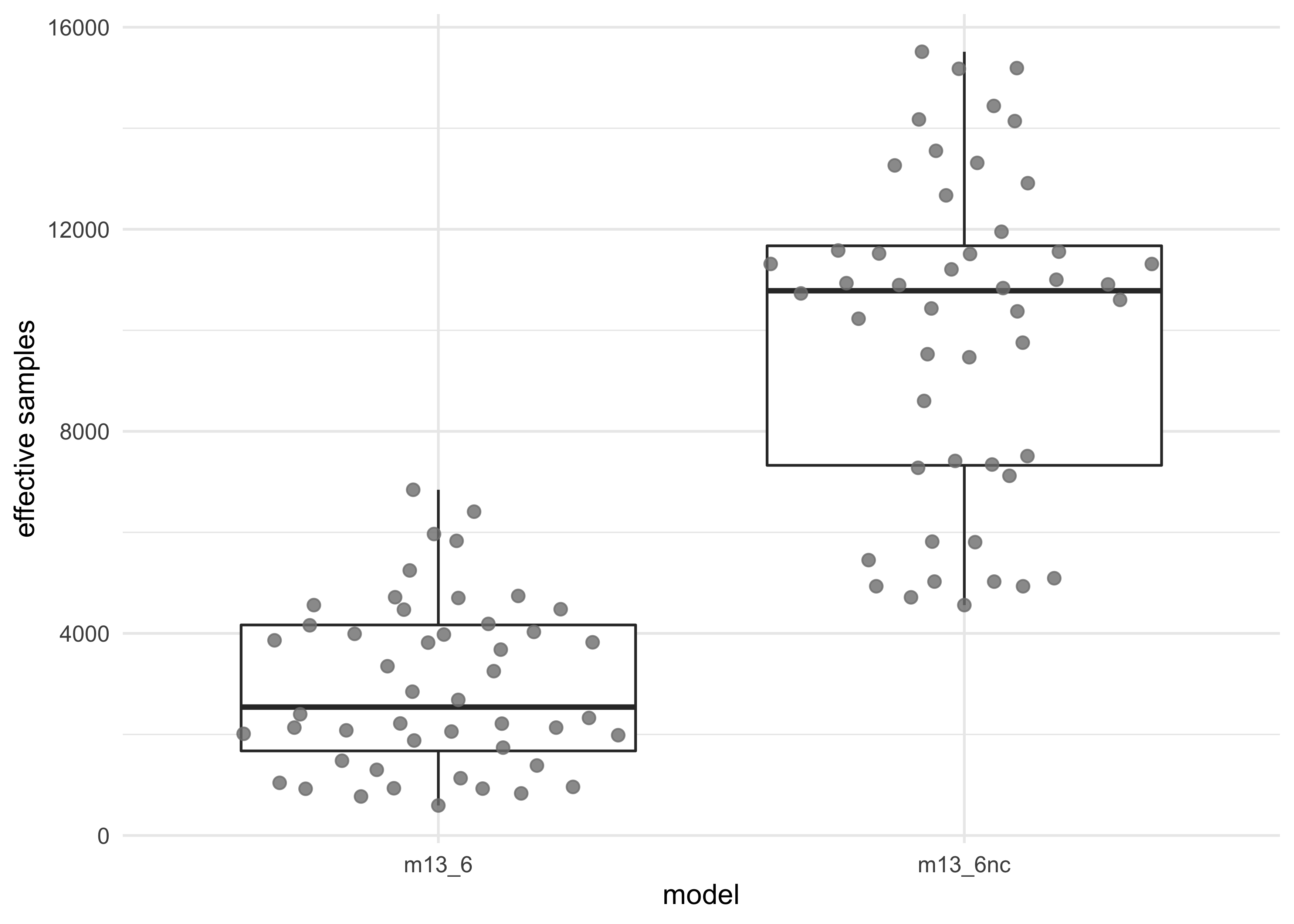
• the non-centered parameterization helped by sampling faster and more effectively

get_neff <- function(mdl, depth) {
    x <- precis(mdl, depth = depth)
    neff_idx <- which(x@names == "n_eff")
    x@.Data[neff_idx]
}

tibble(m13_6 = get_neff(m13_6, depth = 2),
       m13_6nc = get_neff(m13_6nc, depth = 2)) %>%
    pivot_longer(tidyselect::everything()) %>%
    unnest(value) %>%
    ggplot(aes(name, value)) +
    geom_boxplot(outlier.shape = NA) +
    ggbeeswarm::geom_quasirandom(color = grey, size = 2, alpha = 0.8) +
    labs(x = "model",
         y = "effective samples")

#> 18 matrix parameters hidden. Use depth=3 to show them.

#> 75 matrix parameters hidden. Use depth=3 to show them.

• can see the number of effective parameters is much smaller than the real number

WAIC(m13_6nc)

#>       WAIC     lppd  penalty  std_err
#> 1 534.7752 -249.032 18.35563 19.88306

• the standard deviation parameters of the random effects provides a measure of how much regularization was applied
  • the first index for each sigma is the varying intercept standard deviation while the other two are the slopes
  • the values are pretty small suggesting there was a good amount of shrinkage

precis(m13_6nc, depth = 2, pars = c("sigma_actor", "sigma_block"))

#>                     mean        sd       5.5%    94.5%    n_eff    Rhat4
#> sigma_actor[1] 2.3327748 0.9056939 1.31285970 3.952849 5816.898 1.000055
#> sigma_actor[2] 0.4537137 0.3627789 0.04461175 1.098381 7510.460 1.000236
#> sigma_actor[3] 0.5205115 0.4761865 0.03924063 1.385698 7414.251 1.000002
#> sigma_block[1] 0.2295740 0.2077322 0.01855211 0.598803 7343.314 1.000648
#> sigma_block[2] 0.5716266 0.4057379 0.07362251 1.274700 4560.184 1.000127
#> sigma_block[3] 0.5032187 0.4180730 0.04109647 1.243568 7119.573 1.000062

• compare the varying slopes model to the simpler varying intercepts model from the previous chapter
  • the results indicate that there isn’t too much difference between the two models
  • meaning there isn’t much difference in the slopes between actor nor block

stash("m12_5", {
    m12_5 <- map2stan(
        alist(
            pulled_left ~ dbinom(1, p),
            logit(p) <- a + a_actor[actor] + a_block[block_id] + (bp + bpc*condition)*prosoc_left,
            a_actor[actor] ~ dnorm(0, sigma_actor),
            a_block[block_id] ~ dnorm(0, sigma_block),
            a ~ dnorm(0, 10),
            bp ~ dnorm(0, 10),
            bpc ~ dnorm(0, 10),
            sigma_actor ~ dcauchy(0, 1),
            sigma_block ~ dcauchy(0, 1)
        ),
        data = d,
        warmup = 1e3,
        iter = 6e3,
        chains = 4
    )
})

#> Loading stashed object.

compare(m13_6nc, m12_5)

#>             WAIC       SE  dWAIC      dSE    pWAIC    weight
#> m12_5   532.4494 19.66977 0.0000       NA 10.29711 0.7618593
#> m13_6nc 534.7752 19.88306 2.3258 4.070507 18.35563 0.2381407

13.4 Continuous categories and the Gaussian process

• so far, all varying intercepts and slopes were defined over discrete, unordered categories
  • now learn how to use continuous dimensions of variation
    • e.g.: age, income, social standing
• Gaussian process regression: method for applying a varying effect to continuous categories
  • estimates a unique intercept/slope for any value in the variable and applies shrinkage to these values
  • simple outline of the process:
    • calculate differences between all data points in the category
    • the model estimates a function for the covariance between pairs of cases at each distance
    • the coviariance function is the generalization of the varying effects approach to continuous categories

13.4.1 Example: Spatial autocorrelation in Oceanic tools

• in previous modeling of the Oceanic societies data, used a binary contact predictor
  • want to make a model that keeps this as a continuous variable
  • many reasons why islands near each other would have similar tools
• the process:
  • define a distance matrix among the societies
  • then estimate how similarity in tool counts depends on geographic distance

data("islandsDistMatrix")
Dmat <- islandsDistMatrix
colnames(Dmat) <- c("Ml","Tiv","SC","Ya","Fi","Tr","Ch","Mn","To","Ha")
round(Dmat, 1)

#>             Ml Tiv  SC  Ya  Fi  Tr  Ch  Mn  To  Ha
#> Malekula   0.0 0.5 0.6 4.4 1.2 2.0 3.2 2.8 1.9 5.7
#> Tikopia    0.5 0.0 0.3 4.2 1.2 2.0 2.9 2.7 2.0 5.3
#> Santa Cruz 0.6 0.3 0.0 3.9 1.6 1.7 2.6 2.4 2.3 5.4
#> Yap        4.4 4.2 3.9 0.0 5.4 2.5 1.6 1.6 6.1 7.2
#> Lau Fiji   1.2 1.2 1.6 5.4 0.0 3.2 4.0 3.9 0.8 4.9
#> Trobriand  2.0 2.0 1.7 2.5 3.2 0.0 1.8 0.8 3.9 6.7
#> Chuuk      3.2 2.9 2.6 1.6 4.0 1.8 0.0 1.2 4.8 5.8
#> Manus      2.8 2.7 2.4 1.6 3.9 0.8 1.2 0.0 4.6 6.7
#> Tonga      1.9 2.0 2.3 6.1 0.8 3.9 4.8 4.6 0.0 5.0
#> Hawaii     5.7 5.3 5.4 7.2 4.9 6.7 5.8 6.7 5.0 0.0

• the likelihood and linear model for this model look the same as before:
  • Poisson likelihood with a varying intercept linear model with a log link function
  • the $\gamma_{\text{society}}$ is the varying intercept
  • regular coefficient for log population
    • determine if accounting for spatial similarity will wash out the association between log population and total number of tools

$$ T_i \sim \text{Poisson}(\lambda_i) $$ $$ \log \lambda_i = \alpha + \gamma_{\text{society}[i]} + \beta_P \log P_i $$

• add in a multivariate prior for the intercepts for the Gaussian process
  • first is the 10-dimensional Gaussian prior for the intercepts
  • $\textbf{K}$ is the covariance matrix between any pairs of societies $i$ and $j$
    • three new parameters: $\eta$, $\rho$, and $\sigma$
    • the Gaussian shape comes from $\exp(-\rho^2 D_{ij}^2)$ where $D_{ij}$ is the distance between societies $i$ and $j$
      • says that the covariance between two societies declines exponentially with the squared distance
      • $\rho$ determines the rate of decline (large = declines rapidly with distance)
      • the distance need not be squared, but usually is because it is often a more realistic model and fits more easily
    • $\eta^2$ is the maximum covariance between two societies $i$ and $j$
    • $\delta_{ij}\sigma^2$ provides for extra covariance beyond $\eta^2$ when $i=j$
      • the function $\delta_{ij}$ is 1 when $i=j$, else 0
      • this only matters if there is more than one data point per group (which there isn’t in the Oceanic example)
      • therefore, $sigma$ describes how the observations for a single category covary

$$ \gamma \sim \text{MVNormal}([0, …, 0], \textbf{K}) $$ $$ \textbf{K}{ij} = \eta^2 \exp(-\rho^2 D{ij}^2) + \delta_{ij}\sigma^2 $$

• the full model
  • create priors for $\eta^2$ and $\rho^2$ because is easier to fit
  • set $\sigma$ as a small constant because it does not get used in this model (see above)

$$ T_i \sim \text{Poisson}(\lambda_i) $$ $$ \log \lambda_i = \alpha + \gamma_{\text{society}[i]} + \beta_P \log P_i $$ $$ \gamma \sim \text{MVNormal}([0, …, 0], \textbf{K}) $$ $$ \textbf{K}_{ij} = \eta^2 \exp(-\rho^2 D_{ij}^2) + \delta_{ij}(0.01) $$ $$ \alpha \sim \text{Normal}(0, 10) $$ $$ \beta_P \sim \text{Normal}(0, 1) $$ $$ \eta^2 \sim \text{HalfCauchy}(0, 1) $$ $$ \rho^2 \sim \text{HalfCauchy}(0, 1) $$

• fit using map2stan()
  • use GPL2() in order to use a squared distance Gaussian process prior

data("Kline2")
d <- as_tibble(Kline2) %>%
    mutate(society = row_number())

stash("m13_7", {
    m13_7 <- map2stan(
        alist(
            total_tools ~ dpois(lambda),
            log(lambda) <- a + g[society] + bp*logpop,
            g[society] ~ GPL2(Dmat, etasq, rhosq, 0.01),
            a ~ dnorm(0, 10),
            bp ~ dnorm(0, 1),
            etasq ~ dcauchy(0, 1),
            rhosq ~ dcauchy(0, 1)
        ),
        data = list(total_tools = d$total_tools,
                    logpop = d$logpop,
                    society = d$society,
                    Dmat = islandsDistMatrix),
        warmup = 2e3, iter = 1e4, chains = 4
    )
})

#> Loading stashed object.

plot(m13_7)

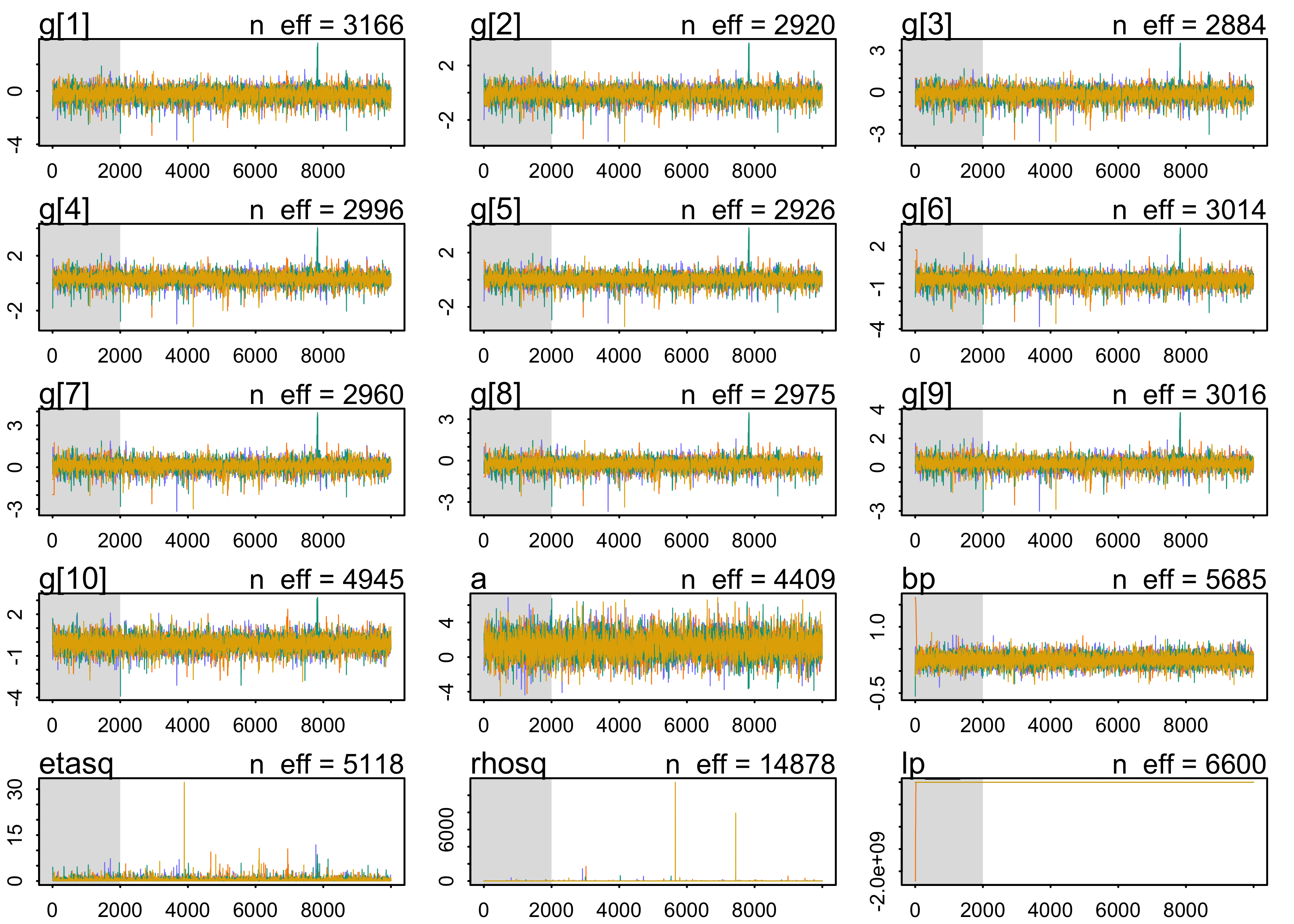
precis(m13_7, depth=2)

#>              mean         sd        5.5%      94.5%     n_eff    Rhat4
#> g[1]  -0.27856102  0.4398912 -0.99830940 0.34423072  3166.290 1.000329
#> g[2]  -0.13030314  0.4275290 -0.82517622 0.48309679  2920.299 1.000473
#> g[3]  -0.17472739  0.4129535 -0.85615406 0.39565329  2883.929 1.000473
#> g[4]   0.29041188  0.3673727 -0.27347655 0.81883438  2996.021 1.000574
#> g[5]   0.01904426  0.3632424 -0.54846932 0.52312820  2925.635 1.000645
#> g[6]  -0.46551126  0.3747591 -1.07984663 0.02455556  3013.954 1.000428
#> g[7]   0.08850494  0.3588191 -0.47706011 0.58111284  2959.900 1.000635
#> g[8]  -0.27052427  0.3616190 -0.84554239 0.21383134  2974.716 1.000614
#> g[9]   0.22699085  0.3398043 -0.28673166 0.70034159  3015.712 1.000794
#> g[10] -0.12811344  0.4518739 -0.83076660 0.55536172  4945.226 1.001099
#> a      1.30857523  1.1568335 -0.49441544 3.17347739  4408.741 1.000326
#> bp     0.24645057  0.1140199  0.06828176 0.42625222  5685.467 1.000516
#> etasq  0.33740391  0.5130216  0.04065684 0.99697571  5117.732 1.000657
#> rhosq  2.81525694 93.1286058  0.05231803 3.80800354 14877.678 1.000069

• interpretation:
  • the coefficient for log population bp is the same as before adding in the Gaussian process for varying intercepts
    • the association between tool counts and population cannot be explained by spatial correlations
• plot posterior of covariance functions using rhosp and etasq samples

post <- extract.samples(m13_7)

median_covar_df <- tibble(etasq = median(post$etasq),
                          rhosq = median(post$rhosq),
                          distance = seq(1, 10, length.out = 100)) %>%
    mutate(density = etasq * exp(-rhosq * distance^2),
           color = "median",
           group = "median")

sample_covar_df <- tibble(etasq = post$etasq[1:100],
                          rhosq = post$rhosq[1:100]) %>%
    mutate(group = as.character(row_number()),
           distance = list(rep(seq(1, 10, length.out = 100), n()))) %>%
    unnest(distance) %>%
    mutate(density = etasq * exp(-rhosq * distance^2),
           color = "posterior samples")

bind_rows(median_covar_df, sample_covar_df) %>%
    ggplot(aes(distance, density)) +
    geom_line(aes(group = group, alpha = color, size = color, color = color)) +
    scale_alpha_manual(values = c(0.8, 0.2)) +
    scale_size_manual(values = c(2, 0.4)) +
    scale_color_manual(values = c(blue, "grey20")) +
    scale_y_continuous(limits = c(0, 1),
                       expand = c(0, 0)) +
    theme(legend.position = c(0.85, 0.7),
          legend.title = element_blank()) +
    labs(x = "distance (thousand km)",
         y = "covariance",
         title = "Posterior distribution of covariance functions")

#> Warning: Removed 11100 row(s) containing missing values (geom_path).

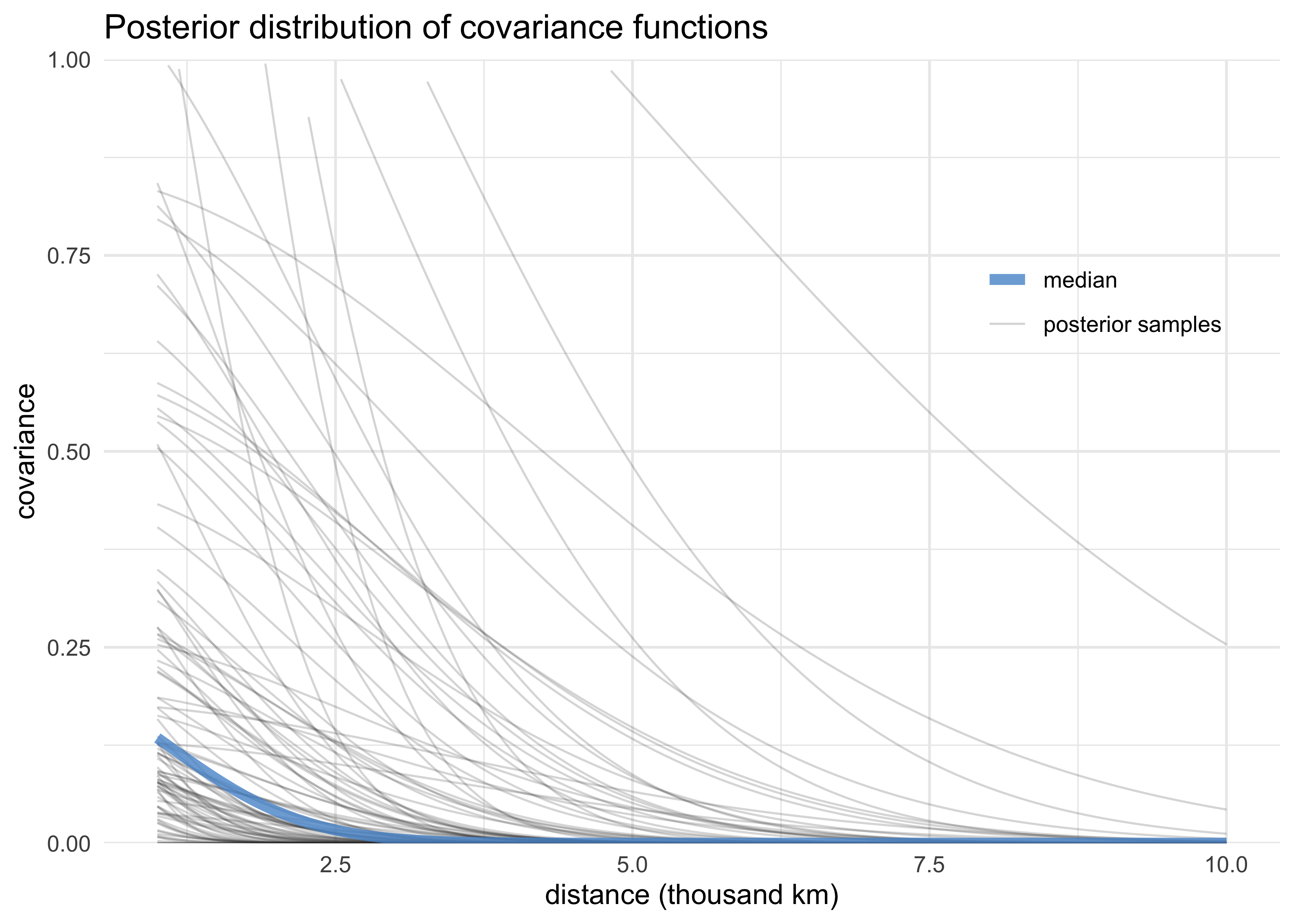
• consider the covariations among societies that are implied by the posterior median
  • first must pass the parameters back through the covariance matrix $\textbf{K}$
  • then convert $\textbf{K}$ to a correlation matrix Rho

# 1. Create the covariance matrix K
K <- matrix(0, nrow = 10, ncol = 10)
for (i in 1:10) {
    for (j in 1:10) {
        K[i,j] <- median(post$etasq) * exp(-median(post$rhosq) * islandsDistMatrix[i,j]^2)
    }
}
diag(K) <- median(post$etasq) + 0.01


# 2. Convert K to a correlation matrix.
Rho <- round(cov2cor(K), 2)
# Add row and column names for convience.
colnames(Rho) <- c("Ml", "Ti", "SC", "Ya", "Fi", "Tr", "Ch", "Mn", "To", "Ha")
rownames(Rho) <- colnames(Rho)
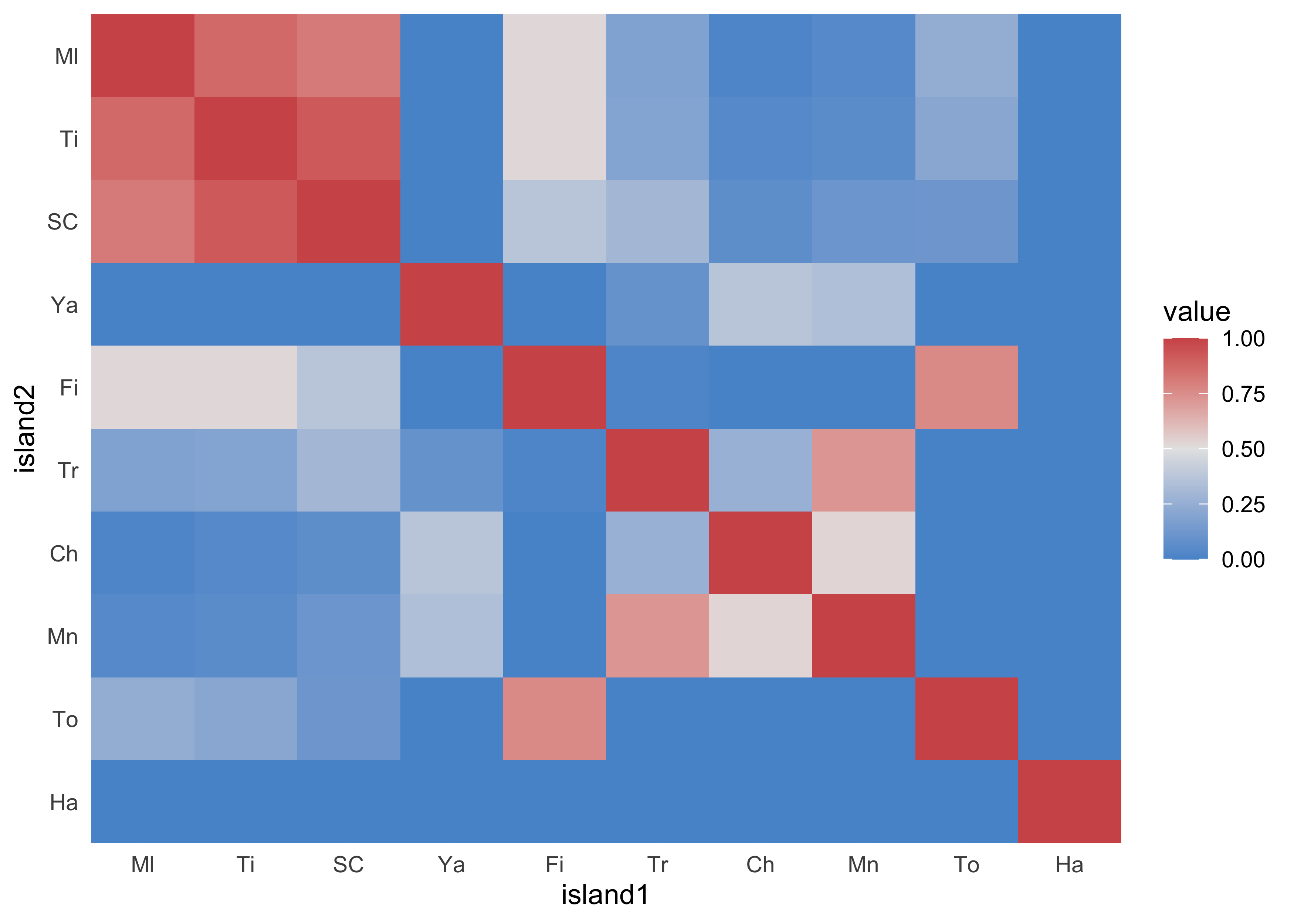
Rho

#>      Ml   Ti   SC   Ya   Fi   Tr   Ch   Mn   To Ha
#> Ml 1.00 0.87 0.81 0.00 0.52 0.18 0.02 0.04 0.24  0
#> Ti 0.87 1.00 0.92 0.00 0.52 0.19 0.04 0.06 0.21  0
#> SC 0.81 0.92 1.00 0.00 0.37 0.30 0.07 0.11 0.12  0
#> Ya 0.00 0.00 0.00 1.00 0.00 0.09 0.37 0.34 0.00  0
#> Fi 0.52 0.52 0.37 0.00 1.00 0.02 0.00 0.00 0.76  0
#> Tr 0.18 0.19 0.30 0.09 0.02 1.00 0.26 0.72 0.00  0
#> Ch 0.02 0.04 0.07 0.37 0.00 0.26 1.00 0.53 0.00  0
#> Mn 0.04 0.06 0.11 0.34 0.00 0.72 0.53 1.00 0.00  0
#> To 0.24 0.21 0.12 0.00 0.76 0.00 0.00 0.00 1.00  0
#> Ha 0.00 0.00 0.00 0.00 0.00 0.00 0.00 0.00 0.00  1

• a cluster of highly correlative islands Ml, Ti, and SC

long_Rho <- Rho %>%
    as.data.frame() %>%
    rownames_to_column(var = "island1") %>%
    as_tibble() %>%
    mutate(island1 = fct_inorder(island1)) %>%
    pivot_longer(-island1, names_to = "island2") %>%
    mutate(island2 = factor(island2, levels = levels(island1)),
           island2 = fct_rev(island2)) 
long_Rho %>%
    ggplot(aes(island1, island2)) +
    geom_tile(aes(fill = value)) +
    scale_fill_gradient2(low = blue, mid = "grey90", high = red, midpoint = 0.5) +
    scale_x_discrete(expand = c(0, 0)) +
    scale_y_discrete(expand = c(0, 0))

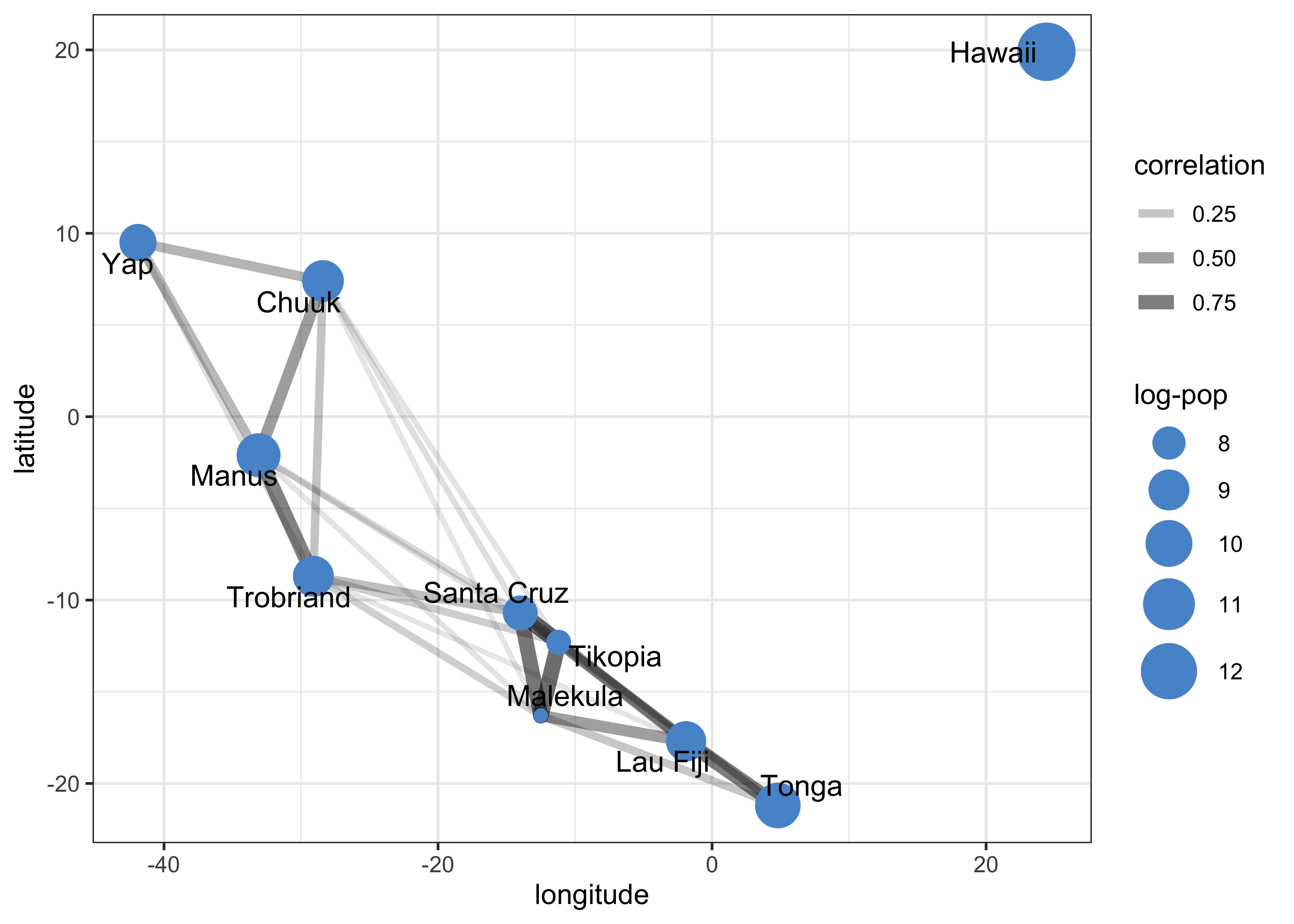
Rho_gr <- as_tbl_graph(Rho, directed = FALSE) %N>%
    left_join(d %>% mutate(name = colnames(Rho)), 
              by = "name")
gr_layout <- create_layout(Rho_gr, layout = "nicely")
gr_layout$x <- d$lon2[match(colnames(Rho), gr_layout$name)]
gr_layout$y <- d$lat[match(colnames(Rho), gr_layout$name)]

ggraph(gr_layout) +
    geom_edge_link(aes(alpha = weight, width = weight),
                   lineend = "round", linejoin = "round") +
    geom_node_point(aes(size = logpop), color = blue) +
    geom_node_text(aes(label = culture), repel = TRUE, size = 4) +
    scale_edge_width_continuous(range = c(1, 3)) +
    scale_edge_alpha_continuous(range = c(0.1, 0.6)) +
    scale_size_continuous(range = c(2, 10)) +
    theme_bw() +
    labs(x = "longitude",
         y = "latitude",
         size = "log-pop",
         edge_width = "correlation",
         edge_alpha = "correlation")

logpop_seq <- seq(6, 14, length.out = 50)
lambda <- map(logpop_seq, ~ exp(post$a + post$b*.x))
lambda_median <- map_dbl(lambda, median)
lambda_pi80 <- map(lambda, PI, prob = 0.80) %>% 
    map_dfr(pi_to_df)

post_pred <- tibble(logpop = logpop_seq,
                    lambda_median = lambda_median) %>%
    bind_cols(lambda_pi80) %>%
    mutate(x10_percent = map_dbl(x10_percent, ~ max(c(.x, 10))),
           x90_percent = map_dbl(x90_percent, ~ min(c(.x, 75))))

gr_layout <- create_layout(Rho_gr, layout = "nicely")
gr_layout$x <- d$logpop[match(colnames(Rho), gr_layout$name)]
gr_layout$y <- d$total_tools[match(colnames(Rho), gr_layout$name)]

ggraph(gr_layout) +
    geom_ribbon((aes(x = logpop, ymin = x10_percent, ymax = x90_percent)),
                data = post_pred,
                alpha = 0.1) +
    geom_line(aes(x = logpop, y = lambda_median),
              data = post_pred,
              color = grey, size = 1, alpha = 0.7, lty = 2) +
    geom_edge_link(aes(alpha = weight, width = weight),
                   lineend = "round", linejoin = "round") +
    geom_node_point(aes(size = logpop), color = blue) +
    geom_node_text(aes(label = culture), repel = TRUE, size = 4) +
    scale_edge_width_continuous(range = c(1, 3)) +
    scale_edge_alpha_continuous(range = c(0.1, 0.6)) +
    scale_size_continuous(range = c(2, 10)) +
    scale_x_continuous(limits = c(6, 13), expand = c(0, 0)) +
    scale_y_continuous(limits = c(10, 75), expand = c(0, 0)) +
    theme_bw() +
    labs(x = "log population",
         y = "total tools",
         size = "log-pop",
         edge_width = "correlation",
         edge_alpha = "correlation",
         title = "Association of log-population and total tools, accouting for spatial correlations",
         subtitle = "The dashed line is the median of the posterior prediction of the total tools given the log-population\n(ignoring the spatial variance), surrounded by the 80 PI.")

#> Warning: Removed 11 row(s) containing missing values (geom_path).

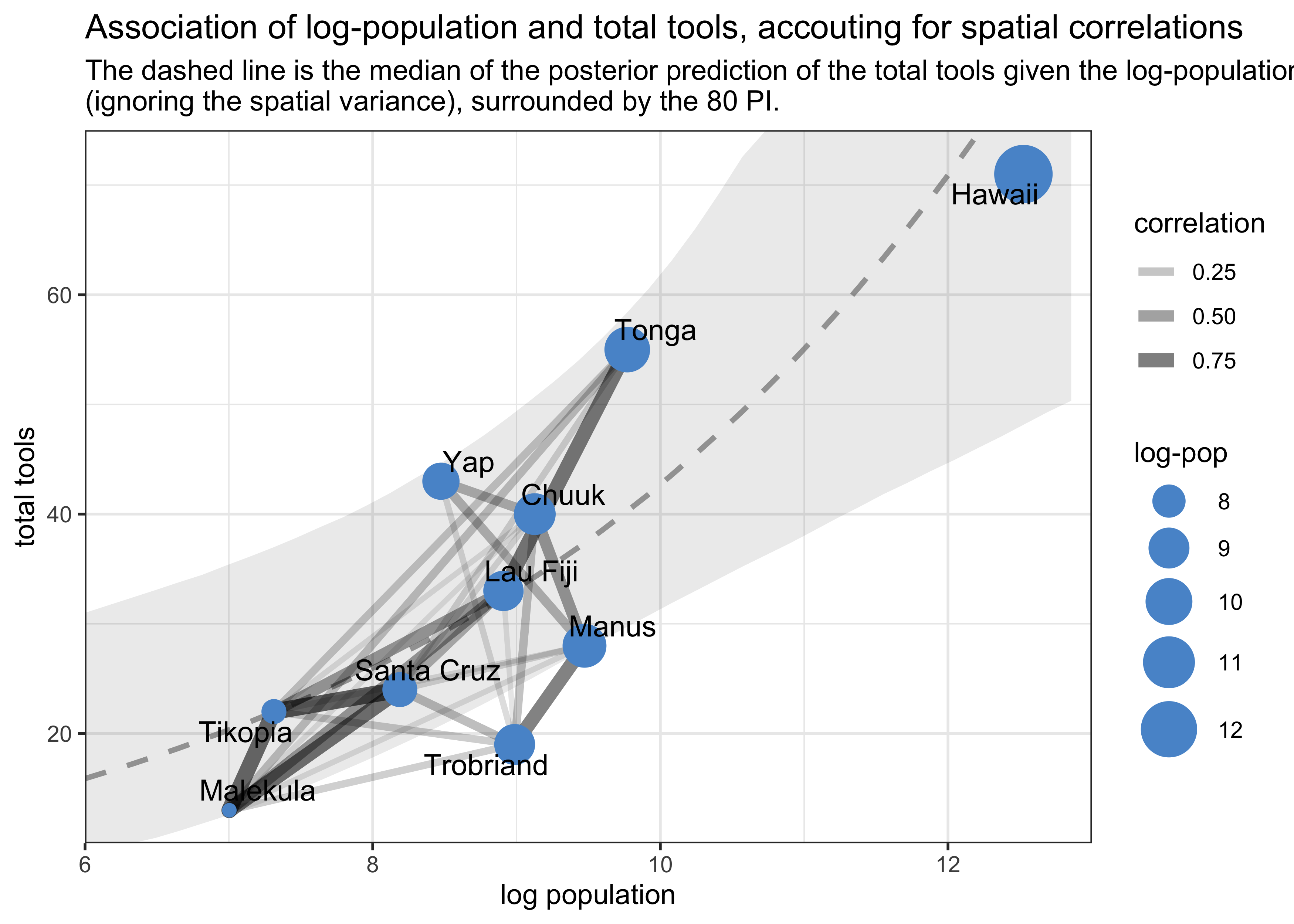
• interpretation of above plots:
  • in the first, we see that Ml, Ti, and SC are all very close together spatially and have a high correlation of their varying intercepts
  • the second shows that these three cultures are below the expected number of tools per their population
    • they they all lie below the expectation and are so close together is consistent with spatial covariance

13.4.2 Other kinds of “distance”

• other examples of a continuous variable for the varying effect:
  • phyolgenetic distance
  • network distance
  • cyclic covariation of time
    • build the covariance matrix with a periodic function such as sine or cosine
• also possible to have more than one dimension of distance in the same model
  • gets merged into a single covariance matrix