Chapter 12. Multilevel Models

Last updated on Jul 1, 2020 23 min read

multi-level models remember features of each cluster in the data as they learn about all of the clusters
- depending on the variation across clusters, the model pools information across clusters
- the pooling improves estimates about each cluster
benefits of the multilevel approach:
1. improved estimates for repeat sampling
2. improved estimates for imbalance in sampling
3. estimates of variation
4. avoid averaging and retain variation
multilevel regression should be the default approach
this chapter starts with the foundations and the following two are more advanced types of multilevel models

12.1 Example: Multilivel tadpoles

example: Reed frog tadpole mortality
- surv: number or survivors
- count: initial number

data("reedfrogs")
d <- as_tibble(reedfrogs)
skimr::skim(d)


Name	d
Number of rows	48
Number of columns	5
_______________________
Column type frequency:
factor	2
numeric	3
________________________
Group variables	None

Data summary

Variable type: factor

skim_variable	n_missing	complete_rate	ordered	n_unique	top_counts
pred	0	1	FALSE	2	no: 24, pre: 24
size	0	1	FALSE	2	big: 24, sma: 24

Variable type: numeric

skim_variable	complete_rate	mean	sd	p0	p25	p50	p75	p100	hist
density	1	23.33	10.38	10.00	10.0	25.00	35.00	35	▇▁▇▁▇
surv	1	16.31	9.88	4.00	9.0	12.50	23.00	35	▇▂▂▂▃
propsurv	1	0.72	0.27	0.11	0.5	0.89	0.92	1	▁▂▂▁▇

there is a lot of variation in the data
- some from experimental treatment, other sources do exist
- each row is a fish tank that is the experimental environment
- each tank is a cluster variable and there are repeated measures from each
- each tank may have a different baseline level of survival, but don’t want to treat them as completely unrelated
  - a dummy variable for each tank would be the wrong solution
varying intercepts model: a multilevel model that estimates an intercept for each tank and the variation among tanks
- for each cluster in the data, use a unique intercept parameter, adaptively learning the prior common to all of the intercepts
- what is learned about each cluster informs all the other clusters
model for predicting tadpole mortality in each tank (nothing new)

$$ s_i \sim \text{Binomial}(n_i, p_i) $$ $$ \text{logit}(p_i) = \alpha_{\text{tank}[i]} $$ $$ \alpha_{\text{tank}} \sim \text{Normal}(0, 5) $$ $$ $$

d$tank <- 1:nrow(d)

stash("m12_1", {
    m12_1 <- map2stan(
        alist(
            surv ~ dbinom(density, p),
            logit(p) <- a_tank[tank],
            a_tank[tank] ~ dnorm(0, 5)
        ),
        data = d
    )
})

#> Loading stashed object.

print(m12_1)

#> map2stan model
#> 1000 samples from 1 chain
#> 
#> Sampling durations (seconds):
#>         warmup sample total
#> chain:1    0.4   0.35  0.75
#> 
#> Formula:
#> surv ~ dbinom(density, p)
#> logit(p) <- a_tank[tank]
#> a_tank[tank] ~ dnorm(0, 5)
#> 
#> WAIC (SE): 1023 (42.9)
#> pWAIC: 49.38

precis(m12_1, depth = 2)

#>                    mean        sd       5.5%      94.5%     n_eff     Rhat4
#> a_tank[1]   2.507409171 1.1524623  0.9310192  4.3793634 1169.7322 1.0026114
#> a_tank[2]   5.612838269 2.7132323  2.1955474 10.5489376  899.3637 1.0008726
#> a_tank[3]   0.955606971 0.7242290 -0.1401785  2.1775927 1460.8578 0.9990305
#> a_tank[4]   5.679923948 2.8455974  2.1598744 10.9713731  699.5095 1.0000048
#> a_tank[5]   2.499838112 1.1727475  0.7699405  4.5863504 1188.1499 1.0000598
#> a_tank[6]   2.517113412 1.1294493  0.9249108  4.4658574 1464.1416 0.9992449
#> a_tank[7]   5.901717876 2.8211771  2.1485777 10.9912848  806.4153 1.0008287
#> a_tank[8]   2.524943494 1.1865708  0.9016065  4.6178622 1326.8743 0.9992859
#> a_tank[9]  -0.434933639 0.6992316 -1.6037425  0.6736126 1861.5726 0.9990238
#> a_tank[10]  2.553526682 1.2725275  0.9580848  4.7399367  811.3452 1.0006649
#> a_tank[11]  0.928007321 0.7012304 -0.1163728  2.0012056 1709.8194 0.9990331
#> a_tank[12]  0.429178891 0.6465231 -0.5735093  1.4651116 1741.1834 0.9991630
#> a_tank[13]  0.920048116 0.7780154 -0.2456616  2.2674043 2287.5157 0.9989996
#> a_tank[14] -0.004138478 0.6422798 -1.0314039  0.9954486 2099.6606 0.9996044
#> a_tank[15]  2.534309631 1.1870475  0.9453520  4.6536340 1017.3940 0.9990010
#> a_tank[16]  2.562492002 1.1979390  0.9383206  4.6150822  904.8553 0.9993926
#>  [ reached 'max' / getOption("max.print") -- omitted 32 rows ]

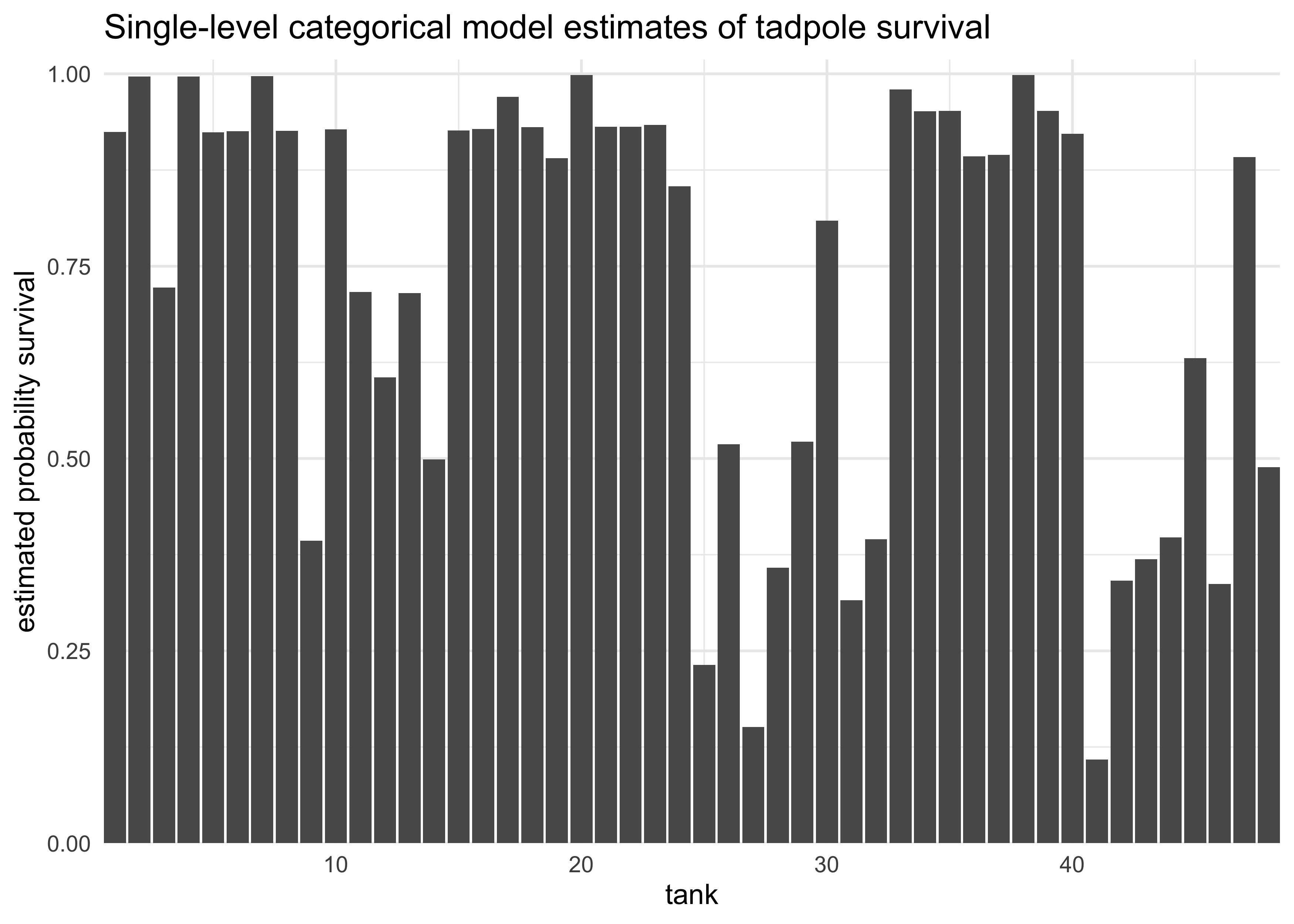
can get expected mortality for each tank by taking the logistic of the coefficients

logistic(coef(m12_1)) %>%
    enframe() %>%
    mutate(name = str_remove_all(name, "a_tank\$$|\$$"),
           name = as.numeric(name)) %>%
    ggplot(aes(x = name, y = value)) +
    geom_col() +
    scale_x_continuous(expand = c(0, 0)) +
    scale_y_continuous(expand = expansion(mult = c(0, 0.02))) +
    labs(x = "tank",
         y = "estimated probability survival",
         title = "Single-level categorical model estimates of tadpole survival")

fit a multilevel model by adding a prior for the a_tank parameters as a function of its own parameters
- now the priors have prior distributions, creating two levels of priors

$$ s_i \sim \text{Binomial}(n_i, p_i) $$ $$ \text{logit}(p_i) = \alpha_{\text{tank}[i]} $$ $$ \alpha_{\text{tank}} \sim \text{Normal}(\alpha, \sigma) $$ $$ \alpha \sim \text{Normal}(0, 1) $$ $$ \sigma \sim \text{HalfCauchy}(0, 1) $$

stash("m12_2", {
    m12_2 <- map2stan(
        alist(
            surv ~ dbinom(density, p),
            logit(p) <- a_tank[tank],
            a_tank[tank] ~ dnorm(a, sigma),
            a ~ dnorm(0, 1),
            sigma ~ dcauchy(0, 1)
        ),
        data = d,
        iter = 4000,
        chains = 4,
        cores = 1
    )
})

#> Loading stashed object.

print(m12_2)

#> map2stan model
#> 8000 samples from 4 chains
#> 
#> Sampling durations (seconds):
#>         warmup sample total
#> chain:1   0.49   0.57  1.06
#> chain:2   0.96   0.80  1.77
#> chain:3   0.81   0.78  1.59
#> chain:4   0.86   0.79  1.65
#> 
#> Formula:
#> surv ~ dbinom(density, p)
#> logit(p) <- a_tank[tank]
#> a_tank[tank] ~ dnorm(a, sigma)
#> a ~ dnorm(0, 1)
#> sigma ~ dcauchy(0, 1)
#> 
#> WAIC (SE): 1010 (37.9)
#> pWAIC: 37.83

precis(m12_2, depth = 2)

#>                  mean        sd        5.5%     94.5%    n_eff     Rhat4
#> a_tank[1]   2.1157682 0.8639729  0.85470075 3.5960058 12139.08 0.9998409
#> a_tank[2]   3.0669080 1.1168484  1.47355820 4.9864858 10998.05 0.9995613
#> a_tank[3]   0.9913351 0.6786515 -0.05967850 2.1209062 15763.42 0.9997261
#> a_tank[4]   3.0461374 1.1196130  1.42470945 4.9792648 11298.69 0.9997267
#> a_tank[5]   2.1296066 0.8687028  0.84447299 3.6169937 14282.14 0.9997553
#> a_tank[6]   2.1356804 0.8839724  0.84089789 3.6140100 13062.73 0.9997334
#> a_tank[7]   3.0432717 1.1007268  1.47339067 4.9349950 11197.91 0.9995695
#> a_tank[8]   2.1174578 0.8736278  0.84567072 3.6043714 13690.49 0.9996902
#> a_tank[9]  -0.1801081 0.6016949 -1.15426295 0.7651194 17013.37 0.9996434
#> a_tank[10]  2.1222757 0.8745242  0.83836130 3.6369076 11732.00 0.9998723
#> a_tank[11]  1.0005859 0.6720581 -0.04092572 2.0949262 16403.51 0.9999348
#> a_tank[12]  0.5737242 0.6156076 -0.39848147 1.5714115 17386.07 1.0000767
#> a_tank[13]  0.9925635 0.6643335 -0.03262575 2.0959440 14427.52 0.9996798
#> a_tank[14]  0.1937834 0.6183100 -0.78266182 1.1916493 17018.95 0.9997141
#> a_tank[15]  2.1205258 0.8764071  0.82664938 3.5924005 13884.02 0.9996914
#> a_tank[16]  2.1278411 0.8625659  0.85117774 3.6198355 13911.59 0.9997513
#>  [ reached 'max' / getOption("max.print") -- omitted 34 rows ]

interpretation:
- $\alpha$: one overall sample intercept
- $\sigma$: variance among tanks
- 48 per-tank intercepts

compare(m12_1, m12_2)

#>           WAIC       SE  dWAIC      dSE    pWAIC      weight
#> m12_2 1009.876 37.94391  0.000       NA 37.83139 0.998797924
#> m12_1 1023.321 42.90494 13.445 6.642773 49.38454 0.001202076

from the comparison, see that the multilevel model only has ~38 effective parameters
- 12 fewer than the single-level model because the prior assigned to each intercept shrinks them all towards the mean $\alpha$
  - $\alpha$ is acting like a regularizing prior, but it has been learned from the data
plot and compare the posterior medians from both models

post <- extract.samples(m12_2)

d %>%
    mutate(propsurv_estimate = logistic(apply(post$a_tank, 2, median)),
           pop_size = case_when(
               density == 10 ~ "small tank",
               density == 25 ~ "medium tank",
               density == 35 ~ "large tank"
           ),
           pop_size = fct_reorder(pop_size, density)) %>%
    ggplot(aes(tank)) +
    facet_wrap(~ pop_size, nrow = 1, scales = "free_x") +
    geom_hline(yintercept = logistic(median(post$a)), 
               lty = 2, color = dark_grey) +
    geom_linerange(aes(x = tank, ymin = propsurv, ymax = propsurv_estimate), 
                   color = light_grey, size = 1) +
    geom_point(aes(y = propsurv), 
               color = grey, size = 1) +
    geom_point(aes(y = propsurv_estimate), 
               color = purple, size = 1) +
    labs(x = "tank",
         y = "proportion surivival",
         title = "Propotion of survival among tadpoles from different tanks.")

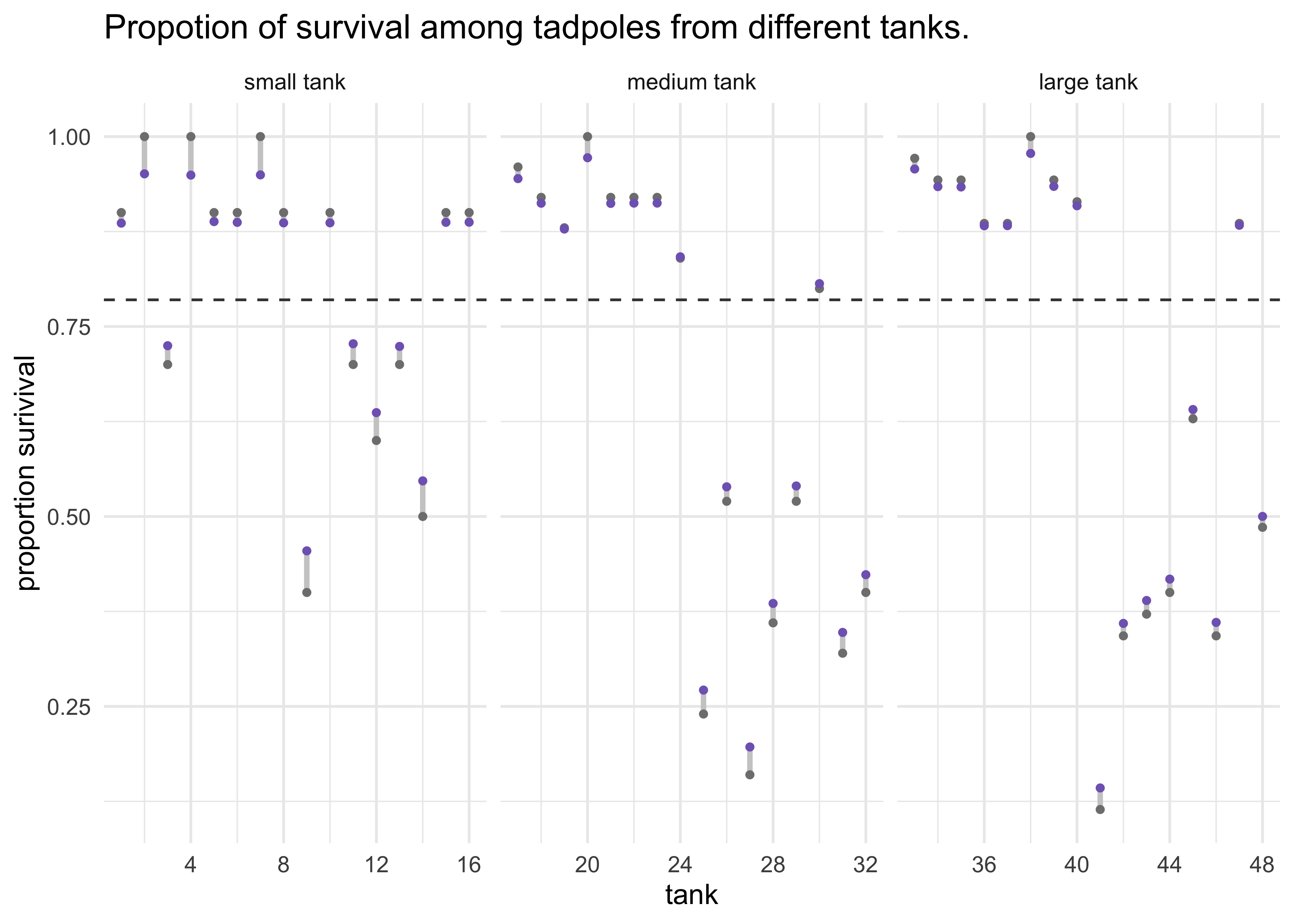
comments on above plot:
- note that all of the purple points $\alpha_\text{tank}$ are skewed towards to the dashed line $\alpha$
  - this is often called shrinkage and comes from regularization
- note that the smaller tanks have shifted more than in the larger tanks
  - there are fewer starting tadpoles, so the shrinkage has a stronger effect
- the shift of the purple points is large the further the empirical value (grey points) are from the dashed line $\alpha$
sample from the posterior distributions:
- first plot 100 Gaussian distributions from samples of the posteriors for $\alpha$ and $\sigma$
- then sample 8000 new log-odds of survival for individual tanks

x <- seq(-3, 5, length.out = 300)
log_odds_gaussian_samples <- map_dfr(1:100, function(i) {
    tibble(i, x, prob = dnorm(x, post$a[i], post$sigma[i]))
})

p1 <- log_odds_gaussian_samples %>%
    ggplot(aes(x, prob, group = factor(i))) +
    geom_line(alpha = 0.5, size = 0.1) +
    labs(x = "log-odds survival",
         y = "density",
         title = "Sampled probability density curves")

p2 <- tibble(sim_tanks = logistic(rnorm(8000, post$a, post$sigma))) %>%
    ggplot(aes(sim_tanks)) +
    geom_density(size = 1, fill = grey, alpha = 0.5) +
    scale_x_continuous(expand = c(0, 0)) +
    scale_y_continuous(expand = expansion(mult = c(0, 0.02))) +
    labs(x = "probability survive",
         y = "density",
         title = "Simulated survival proportions")

p1 | p2

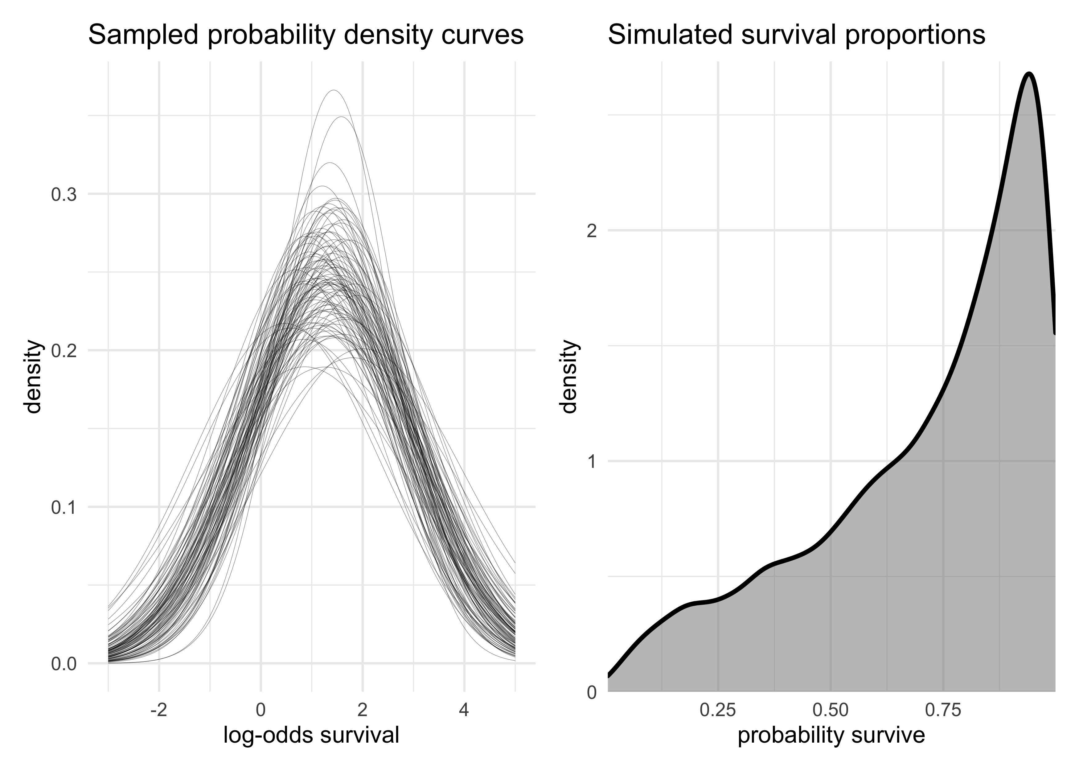
there is uncertainty about both the location $\alpha$ and scale $\sigma$ of the population distribution of log-odds of survival
- this uncertainty is propagated into the simulated probabilities of survival

12.2 Varying effects and the underfitting/overfitting trade-off

“Varying intercepts are just regularized estimates, but adaptivelyy regulraized by estimating how diverse the cluster are while estimating the features of each cluster.”
- varying effect estimates are more accurate estimates of the individual cluster intercepts
partial pooling helps prevent overfitting and underfitting
- pooling all of the tanks into a single intercept would make an underfit model
- having completely separate intercepts for each tank would overfit
demonstration: simulate tadpole data so we know the true per-pond survival probabilities
- this is also a demonstration of the important skill of simulation and model validation

12.2.1 The model

we will use the same multilevel binomial model as before (using “ponds” instead of “tanks”)

$$ s_i \sim \text{Binomial}(n_i, p_i) $$ $$ \text{logit}(p_i) = \alpha_{\text{pond[i]}} $$ $$ \alpha_\text{pond} \sim \text{Normal}(\alpha, \sigma) $$ $$ \alpha \sim \text{Normal}(0, 1) $$ $$ \sigma \sim \text{HalfCauchy}(0, 1) $$ - need to assign values for: * $\alpha$: the average log-odds of survival for all of the ponds * $\sigma$: the standard deviation of the distribution of log-odds of survival among ponds * $\alpha_\text{pond}$: the individual pond intercepts * $n_i$: the number of tadpoles per pond

12.2.2 Assign values to the parameters

steps in code:
1. initialize $\alpha$, $\sigma$, number of ponds, number of tadpoles per ponds
2. use these parameters to generate $\alpha_\text{pond}$
3. put data into a data frame

set.seed(0)

# 1. Initialize top level parameters.
a <- 1.4
sigma <- 1.5
nponds <- 60
ni <- as.integer(rep(c(5, 10, 25, 35), each = 15))

# 2. Sample second level parameters for each pond.
a_pond <- rnorm(nponds, mean = a, sd = sigma)

# 3. Organize into a data frame.
dsim <- tibble(pond = seq(1, nponds), 
               ni = ni,
               true_a = a_pond)
dsim

#> # A tibble: 60 x 3
#>     pond    ni   true_a
#>    <int> <int>    <dbl>
#>  1     1     5  3.29   
#>  2     2     5  0.911  
#>  3     3     5  3.39   
#>  4     4     5  3.31   
#>  5     5     5  2.02   
#>  6     6     5 -0.910  
#>  7     7     5  0.00715
#>  8     8     5  0.958  
#>  9     9     5  1.39   
#> 10    10     5  5.01   
#> # … with 50 more rows

12.2.3 Simulate survivors

simulate the binomial survival process
- each pond $i$ has $n_i$ potential survivors with probability of survival $p_i$
- from the model definition (using the logit link function), $p_i$ is:

$$ p_i = \frac{\exp(\alpha_i)}{1 + \exp(\alpha_i)} $$

dsim$si <- rbinom(nponds, 
                  prob = logistic(dsim$true_a), 
                  size = dsim$ni)

12.2.4 Compute the no-pooling estiamtes

the estimates from not pooling information across ponds is the same as calculating the proportion of survivors in each pond
- would get same values if used a dummy variable for each pond and weak priors
calculate these value and keep on the probability scale

dsim$p_nopool <- dsim$si / dsim$ni

12.2.5 Compute the partial-pooling estimates

now fit the multilevel model

stash("m12_3", {
    m12_3 <- map2stan(
        alist(
            si ~ dbinom(ni, p),
            logit(p) <- a_pond[pond],
            a_pond[pond] ~ dnorm(a, sigma),
            a ~ dnorm(0, 1),
            sigma ~ dcauchy(0, 1)
        ),
        data = dsim,
        iter = 1e4,
        warmup = 1000
    )
})

#> Loading stashed object.

precis(m12_3, depth = 2)

#>                  mean        sd       5.5%     94.5%     n_eff     Rhat4
#> a_pond[1]   2.5053151 1.1125019  0.8842713 4.4213093  9633.975 0.9999010
#> a_pond[2]  -0.4977377 0.8163556 -1.8456079 0.7864969 13954.284 0.9999419
#> a_pond[3]   2.4900753 1.0993925  0.8644481 4.3488823 11543.637 1.0000289
#> a_pond[4]   2.5089798 1.1186088  0.8810598 4.4225452  8439.085 0.9999777
#> a_pond[5]   2.5067354 1.1084190  0.8990796 4.4121802  8900.319 0.9999229
#> a_pond[6]   0.1340153 0.7981828 -1.1291088 1.3944146 15656.275 1.0004159
#> a_pond[7]   0.7728565 0.8203942 -0.5035563 2.1126640 13286.103 0.9998930
#> a_pond[8]   1.5282302 0.9254883  0.1451402 3.0931019 11202.035 0.9998956
#> a_pond[9]   2.5097866 1.1005938  0.8965482 4.3920475  8239.384 1.0000038
#> a_pond[10]  2.4819890 1.1084175  0.8572985 4.3915817 12718.861 0.9999360
#> a_pond[11]  2.4793137 1.0892989  0.8863951 4.2945049  9759.468 1.0000382
#> a_pond[12]  0.7757112 0.8560909 -0.5276722 2.1640762 13023.329 0.9998889
#> a_pond[13] -0.4880659 0.8266811 -1.8513618 0.8007399 13347.095 1.0002797
#> a_pond[14]  2.4953084 1.0840919  0.8978628 4.3287307 10575.209 0.9998917
#> a_pond[15]  0.7641494 0.8234787 -0.5361413 2.1129975 13176.483 0.9999043
#> a_pond[16]  0.2485980 0.6022535 -0.7145539 1.2187904 17888.678 0.9999321
#>  [ reached 'max' / getOption("max.print") -- omitted 46 rows ]

compute the predicted survival proportions

estimated_a_pond <- as.numeric(coef(m12_3)[1:nponds])
dsim$p_partpool <- logistic(estimated_a_pond)

compute known survival proportions from the real $\alpha_\text{pond}$ values

dsim$p_true <- logistic(dsim$true_a)

plot the results and compute error between the estimated and true varying effects

dsim %>%
    transmute(nopool_error = abs(p_nopool - p_true),
              partpool_error = abs(p_partpool - p_true),
              pond, ni) %>%
    pivot_longer(-c(pond, ni),
                 names_to = "model_type", values_to = "absolute_error") %>%
    group_by(ni, model_type) %>%
    mutate(avg_error = mean(absolute_error)) %>%
    ungroup() %>%
    ggplot(aes(x = pond, y = absolute_error)) +
    facet_wrap(~ ni, scales = "free_x", nrow = 1) +
    geom_line(aes(y = avg_error, color = model_type, group = model_type), size = 1.5, alpha = 0.7) +
    geom_line(aes(group = factor(pond)), color = light_grey, size = 0.8) +
    geom_point(aes(color = model_type)) +
    scale_color_brewer(palette = "Dark2") +
    theme(legend.position = c(0.9, 0.7)) +
    labs(x = "pond number",
         y = "absolute error",
         color = "model type",
         title = "Comparing the error between estimates from amnesiac and multilevel models")

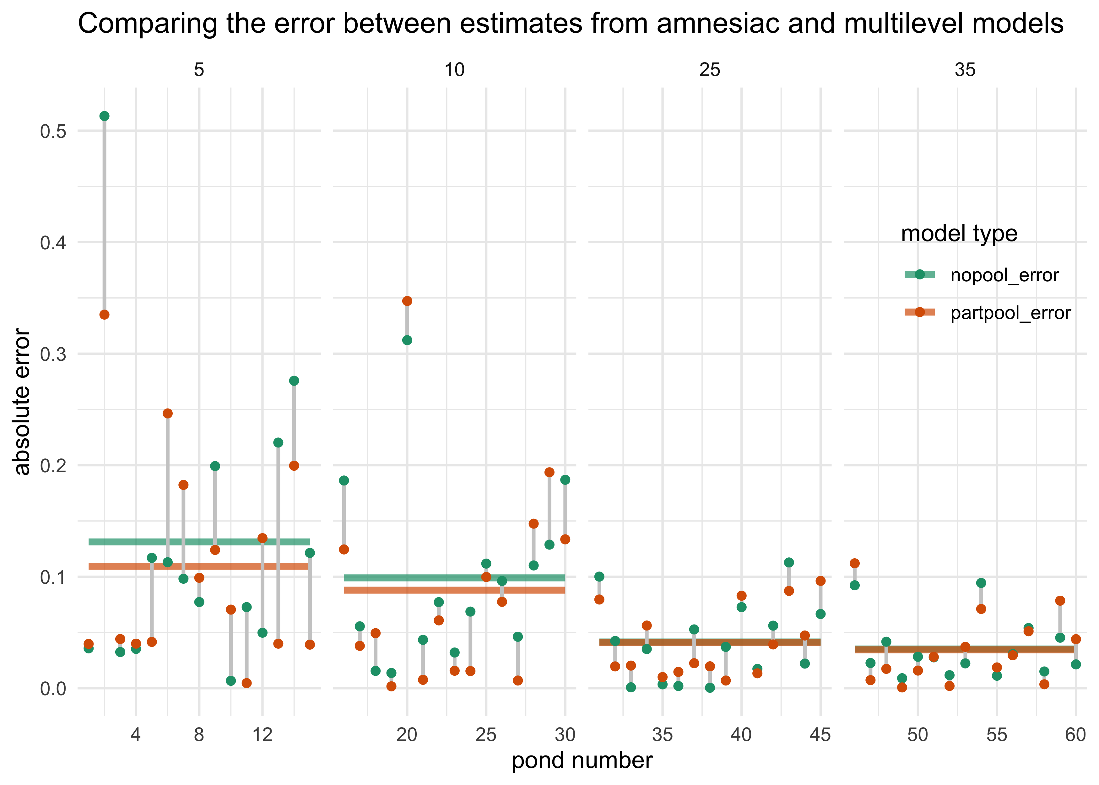
interpretation:
- both models perform better with larger ponds becasue more data
- the partial pooling model performs better, on average, than the no pooling model

12.3 More than one type of cluster

often are multiple clusters of data in the same model
example: chimpanzee data
- one block for each chimp
- one block for each day of testing

12.3.1 Multilevel chimpanzees

similar model as before
- add varying intercepts for actor
- put both the $\alpha$ and $\alpha_\text{actor}$ in the linear model
  - it is to allow for adding other varying effects
  - instead of having $\alpha$ as the mean for $\alpha_\text{actor}$, the mean for $\alpha_\text{actor} = 0$ and the mean $\alpha$ is in the linear model instead

$$ L_i \sim \text{Binomial}(1, p_i) $$ $$ \text{logit}(p_i) = \alpha + \alpha_{\text{actor}[i]} + (\beta_P + \beta_{PC} C_i) P_i $$ $$ \alpha_\text{actor} \sim \text{Normal}(0, \sigma_\text{actor}) $$ $$ \alpha \sim \text{Normal}(0, 10) $$ $$ \beta_P \sim \text{Normal}(0, 10) $$ $$ \beta_{PC} \sim \text{Normal}(0, 10) $$ $$ \alpha_\text{actor} \sim \text{HalfCauchy}(0, 1) $$ $$ $$

data("chimpanzees")
d <- as_tibble(chimpanzees) %>%
    select(-recipient)

stash("m12_4", {
    m12_4 <- map2stan(
        alist(
            pulled_left ~ dbinom(1, p),
            logit(p) <- a + a_actor[actor] + (bp + bpc*condition)*prosoc_left,
            a_actor[actor] ~ dnorm(0, sigma_actor),
            a ~ dnorm(0, 10),
            bp ~ dnorm(0, 10),
            bpc ~ dnorm(0, 10),
            sigma_actor ~ dcauchy(0, 1)
        ),
        data = d,
        warmup = 1e3,
        iter = 5e3,
        chains = 4
    )
})

#> Loading stashed object.

print(m12_4)

#> map2stan model
#> 16000 samples from 4 chains
#> 
#> Sampling durations (seconds):
#>         warmup sample total
#> chain:1   7.29  21.96 29.25
#> chain:2   7.15  23.66 30.81
#> chain:3   5.73  24.91 30.64
#> chain:4   6.07  20.77 26.85
#> 
#> Formula:
#> pulled_left ~ dbinom(1, p)
#> logit(p) <- a + a_actor[actor] + (bp + bpc * condition) * prosoc_left
#> a_actor[actor] ~ dnorm(0, sigma_actor)
#> a ~ dnorm(0, 10)
#> bp ~ dnorm(0, 10)
#> bpc ~ dnorm(0, 10)
#> sigma_actor ~ dcauchy(0, 1)
#> 
#> WAIC (SE): 531 (19.5)
#> pWAIC: 8.11

precis(m12_4, depth = 2)

#>                   mean        sd       5.5%       94.5%    n_eff     Rhat4
#> a_actor[1]  -1.1735896 1.0012019 -2.7300473  0.23364730 2101.429 1.0012547
#> a_actor[2]   4.2071147 1.7506271  2.1320036  7.05788804 3273.263 1.0003060
#> a_actor[3]  -1.4800454 1.0031659 -3.0516861 -0.05041580 2089.652 1.0013224
#> a_actor[4]  -1.4757774 1.0020223 -3.0374286 -0.05192123 2099.656 1.0013993
#> a_actor[5]  -1.1713944 1.0020717 -2.7413405  0.25875482 2094.726 1.0013656
#> a_actor[6]  -0.2278687 0.9993039 -1.7950471  1.20604520 2102.027 1.0013138
#> a_actor[7]   1.3076865 1.0255852 -0.2800768  2.81614317 2246.178 1.0011328
#> a            0.4576892 0.9800871 -0.9178915  1.99125639 2025.506 1.0013659
#> bp           0.8231619 0.2621824  0.4136777  1.25290336 6494.962 0.9999752
#> bpc         -0.1311277 0.2989366 -0.6053379  0.34261909 6701.342 1.0000421
#> sigma_actor  2.2768974 0.9825956  1.2487228  3.92728797 3201.064 1.0008673

note that the mean population of actors $\alpha$ and the individual deviations from that mean $\alpha_\text{actor}$ must be summed to calculate the entrie intercept: $\alpha + \alpha_\text{actor}$

post <- extract.samples(m12_4)
total_a_actor <- map(1:7, ~ post$a + post$a_actor[, .x])
round(map_dbl(total_a_actor, mean), 2)

#> [1] -0.72  4.66 -1.02 -1.02 -0.71  0.23  1.77

12.3.2 Two types of cluster

add a second cluster on block
- replicate the structure for actor
- keep only a single global mean parameter $\alpha$ and have the varying intercepts with a mean of 0

$$ L_i \sim \text{Binomial}(1, p_i) $$ $$ \text{logit}(p_i) = \alpha + \alpha_{\text{actor}[i]} + \alpha_{\text{block}[i]} + (\beta_P + \beta_{PC} C_i) P_i $$ $$ \alpha_\text{actor} \sim \text{Normal}(0, \sigma_\text{actor}) $$ $$ \alpha_\text{block} \sim \text{Normal}(0, \sigma_\text{block}) $$ $$ \alpha \sim \text{Normal}(0, 10) $$ $$ \beta_P \sim \text{Normal}(0, 10) $$ $$ \beta_{PC} \sim \text{Normal}(0, 10) $$ $$ \alpha_\text{actor} \sim \text{HalfCauchy}(0, 1) $$ $$ \alpha_\text{block} \sim \text{HalfCauchy}(0, 1) $$ $$ $$

d$block_id <- d$block  # 'block' is a reserved name in Stan.

stash("m12_5", {
    m12_5 <- map2stan(
        alist(
            pulled_left ~ dbinom(1, p),
            logit(p) <- a + a_actor[actor] + a_block[block_id] + (bp + bpc*condition)*prosoc_left,
            a_actor[actor] ~ dnorm(0, sigma_actor),
            a_block[block_id] ~ dnorm(0, sigma_block),
            a ~ dnorm(0, 10),
            bp ~ dnorm(0, 10),
            bpc ~ dnorm(0, 10),
            sigma_actor ~ dcauchy(0, 1),
            sigma_block ~ dcauchy(0, 1)
        ),
        data = d,
        warmup = 1e3,
        iter = 6e3,
        chains = 4
    )
})

#> Loading stashed object.

print(m12_5)

#> map2stan model
#> 20000 samples from 4 chains
#> 
#> Sampling durations (seconds):
#>         warmup sample total
#> chain:1  10.72  35.09 45.81
#> chain:2   7.90  29.20 37.10
#> chain:3   7.56  21.69 29.25
#> chain:4   5.48  26.69 32.18
#> 
#> Formula:
#> pulled_left ~ dbinom(1, p)
#> logit(p) <- a + a_actor[actor] + a_block[block_id] + (bp + bpc * 
#>     condition) * prosoc_left
#> a_actor[actor] ~ dnorm(0, sigma_actor)
#> a_block[block_id] ~ dnorm(0, sigma_block)
#> a ~ dnorm(0, 10)
#> bp ~ dnorm(0, 10)
#> bpc ~ dnorm(0, 10)
#> sigma_actor ~ dcauchy(0, 1)
#> sigma_block ~ dcauchy(0, 1)
#> 
#> WAIC (SE): 532 (19.7)
#> pWAIC: 10.3

precis(m12_5, depth = 2)

#>                    mean        sd       5.5%       94.5%     n_eff     Rhat4
#> a_actor[1] -1.175064397 0.9841238 -2.7606242  0.26572500  3127.582 1.0017434
#> a_actor[2]  4.180714321 1.6729009  2.1251215  6.98239536  4813.958 1.0003135
#> a_actor[3] -1.480590647 0.9832722 -3.0791206 -0.04821499  3130.192 1.0019540
#> a_actor[4] -1.478783548 0.9836902 -3.0794615 -0.05543320  3190.286 1.0018033
#> a_actor[5] -1.174174061 0.9817486 -2.7569231  0.26783679  3081.939 1.0019227
#> a_actor[6] -0.226458711 0.9796456 -1.8242262  1.22181433  3165.682 1.0016978
#> a_actor[7]  1.316572431 1.0070672 -0.2909612  2.82251597  3279.139 1.0016276
#> a_block[1] -0.183995506 0.2313540 -0.6197247  0.07417105  4061.437 1.0011753
#> a_block[2]  0.037069316 0.1877480 -0.2391722  0.34372436 10717.249 1.0002318
#> a_block[3]  0.052974160 0.1866553 -0.2097568  0.37125753  9201.858 1.0001379
#> a_block[4]  0.004609523 0.1835454 -0.2868766  0.29340365 11224.762 1.0003635
#> a_block[5] -0.034560355 0.1870889 -0.3514144  0.23976596 10534.296 1.0004691
#> a_block[6]  0.113814284 0.1999371 -0.1362324  0.48060435  6501.544 1.0003009
#> a           0.456947755 0.9683053 -0.9553192  2.02343452  3019.549 1.0021039
#> bp          0.831444842 0.2628057  0.4108247  1.25433671 11156.767 0.9998428
#> bpc        -0.141912446 0.2989153 -0.6232644  0.33594039 11467.687 1.0000441
#>  [ reached 'max' / getOption("max.print") -- omitted 2 rows ]

there was a warning message, though it can be safely ignored:

There were 11 divergent iterations during sampling. Check the chains (trace plots, n_eff, Rhat) carefully to ensure they are valid.

interpretation:
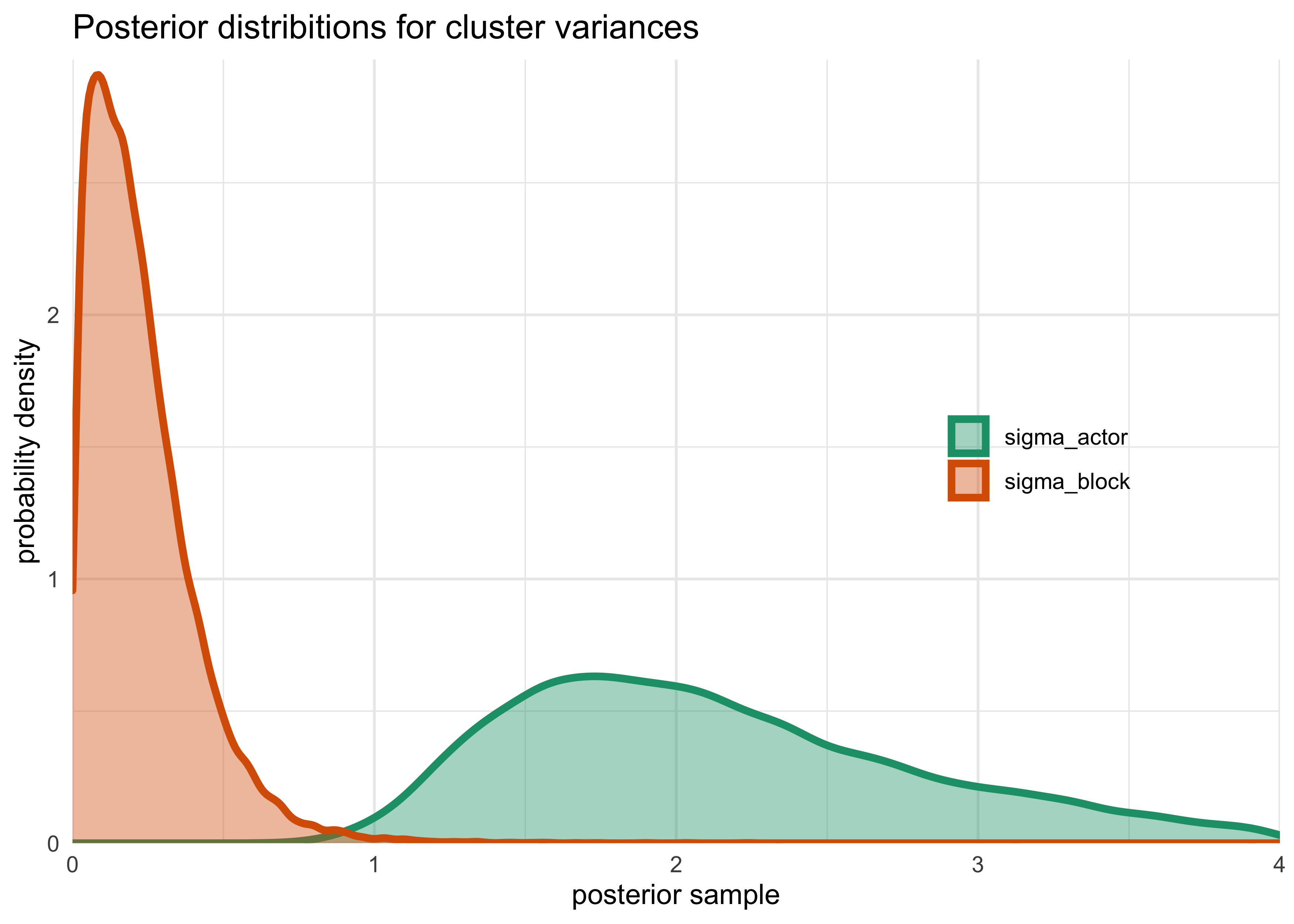
- normal to have variance of n_eff across parameters of these more complex models
- $\sigma_\text{block}$ is much smaller than $\sigma_\text{actor}$ so there is more variation between actors
  - therefore, adding block hasnt added much overfitting risk

post <- extract.samples(m12_5)
enframe(post) %>%
    filter(name %in% c("sigma_actor", "sigma_block")) %>%
    unnest(value) %>%
    ggplot(aes(value)) +
    geom_density(aes(color = name, fill = name), size = 1.4, alpha = 0.4) +
    scale_x_continuous(limits = c(0, 4),
                       expand = c(0, 0)) +
    scale_y_continuous(expand = expansion(mult = c(0, 0.02))) +
    scale_color_brewer(palette = "Dark2") +
    scale_fill_brewer(palette = "Dark2") +
    theme(legend.title = element_blank(),
          legend.position = c(0.8, 0.5)) +
    labs(x = "posterior sample",
         y = "probability density",
         title = "Posterior distribitions for cluster variances")

#> Warning: Removed 986 rows containing non-finite values (stat_density).

compare(m12_4, m12_5)

#>           WAIC       SE   dWAIC      dSE     pWAIC    weight
#> m12_4 531.3511 19.50534 0.00000       NA  8.112905 0.6339337
#> m12_5 532.4494 19.66977 1.09826 1.774829 10.297114 0.3660663

there are 7 more parameters in m12_5 than m12_4, but the pWAIC (effective number of parameters) shows there are only about 2 more effective parameters
- because the variance from block is so low
the models have very close WAIC values because they make very similar predictions
- block had very little influence on the model
- keeping and reporting on both models is important to demonstrate this fact

12.3.3 Even more clusters

MCMC can handle thousands of varying effects
need not be shy to include a varying effect if there is theoretical reason it would introduce variance
- overfitting risk is low as $\sigma$ for the parameters will shrink
- indicates the importance of the cluster

12.4 Multilevel posterior predictions

model checking: a robust way to check the fit of a model is to compare the sample to the posterior predictions
- *information criteria are also useful indicators of model flexibility and risk of overfitting
for a multilevel model:
- should not expect to “retrodict” the sample because shrinkage will distort some predictions
- will want predictions for existing clusters of data and new clusters of data

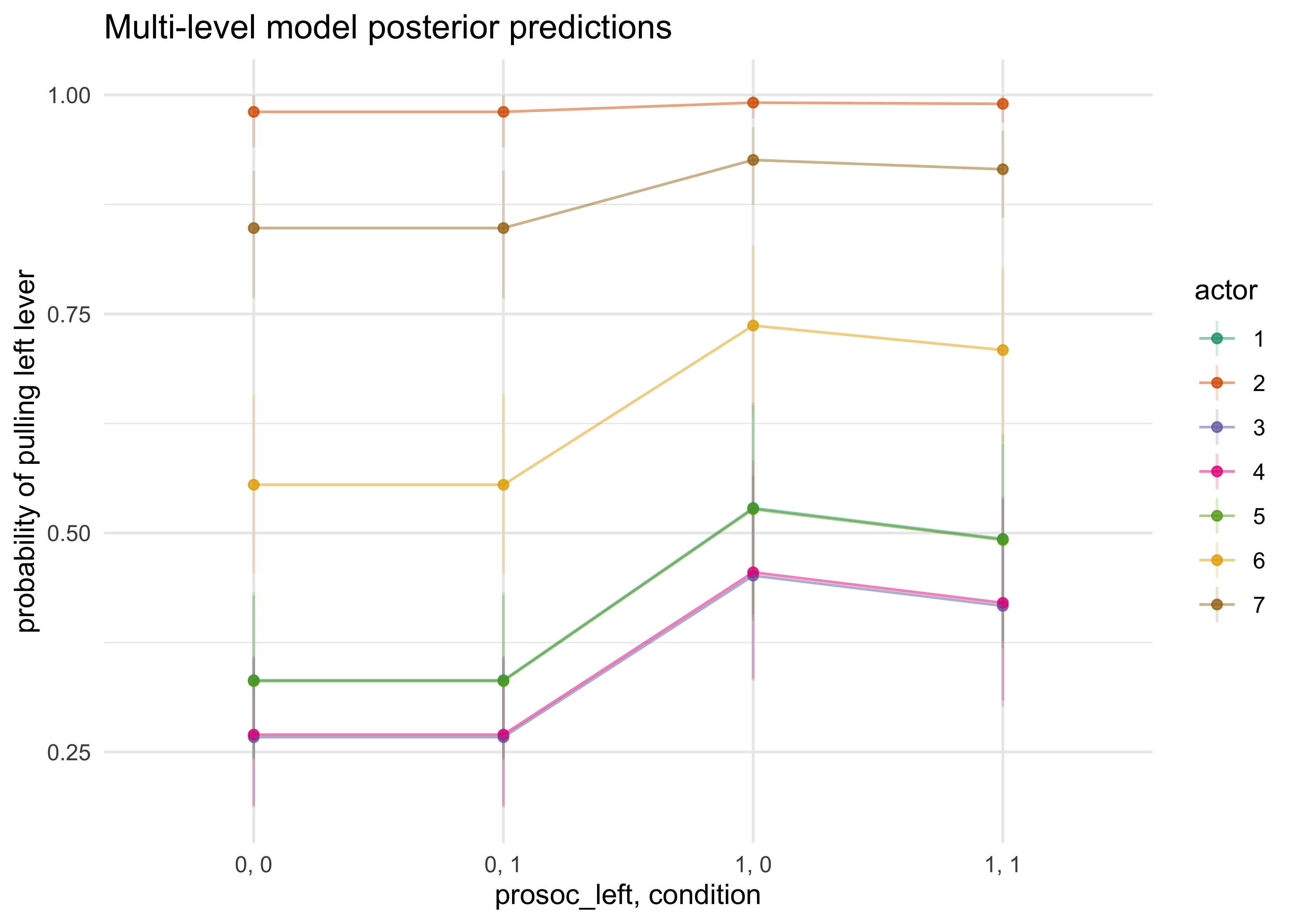
12.4.1 Posterior prediction for same clusters

example uing chimpanzees dataset and model 12_4
- each actor is a cluster of the data

# A data frame of all possible conditions
d_conditions <- tibble(
    prosoc_left = c(0, 1, 0, 1),
    condition = c(0, 0, 1, 1)
)

# A data frame of all possible conditions for each actor (chimp)
d_pred <- tibble(actor = 1:7) %>%
    mutate(data = rep(list(d_conditions), 7)) %>%
    unnest(data)

# make predictions
link_m12_4 <- link(m12_4, data = d_pred)

#> [ 100 / 1000 ][ 200 / 1000 ][ 300 / 1000 ][ 400 / 1000 ][ 500 / 1000 ][ 600 / 1000 ][ 700 / 1000 ][ 800 / 1000 ][ 900 / 1000 ][ 1000 / 1000 ]

d_pred %>%
    mutate(post_pred_mean = apply(link_m12_4, 2, mean)) %>%
    bind_cols(apply(link_m12_4, 2, PI) %>% pi_to_df()) %>%
    mutate(x = paste(prosoc_left, condition, sep = ", ")) %>%
    ggplot(aes(x = x, y = post_pred_mean, color = factor(actor))) +
    geom_linerange(aes(ymin = x5_percent, ymax = x94_percent), alpha = 0.2) +
    geom_point(alpha = 0.8) +
    geom_line(aes(group = factor(actor)), alpha = 0.5) +
    scale_color_brewer(palette = "Dark2") +
    labs(x = "prosoc_left, condition",
         y = "probability of pulling left lever",
         title = "Multi-level model posterior predictions",
         color = "actor")

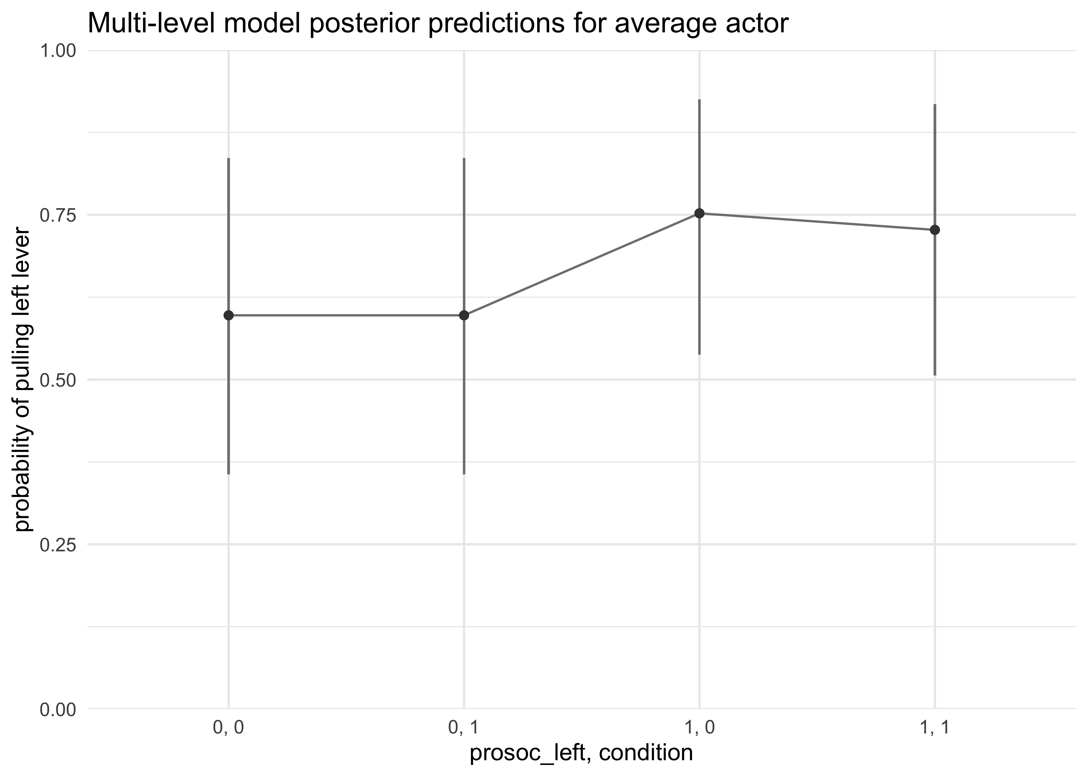
12.4.2 Posterior prediction for new clusters

often we do not care about the individual clusters in the data
- we don’t necessarily want predictions for the 7 chimps in the data, but for all of the species
first attempt: construct a posterior prediciton for the average actor using $\alpha$
- however, does not show the variation among actors

d_pred$actor <- 1  # A non-zero placeholder
a_actor_zeros = matrix(0, nrow = 1e3, ncol = 7)

link_m12_4 <- link(m12_4, n = 1e3, data = d_pred, 
                   replace = list(a_actor = a_actor_zeros))

#> [ 100 / 1000 ][ 200 / 1000 ][ 300 / 1000 ][ 400 / 1000 ][ 500 / 1000 ][ 600 / 1000 ][ 700 / 1000 ][ 800 / 1000 ][ 900 / 1000 ][ 1000 / 1000 ]

d_pred %>%
    mutate(x = paste(prosoc_left, condition, sep = ", "),
           pred_p_mean = apply(link_m12_4, 2, mean)) %>%
    bind_cols(apply(link_m12_4, 2, PI, prob = 0.8) %>% pi_to_df()) %>%
    ggplot(aes(x = x, y = pred_p_mean)) +
    geom_linerange(aes(ymin = x10_percent, ymax = x90_percent), color = grey) +
    geom_line(aes(group = factor(actor)), color = grey) +
    geom_point(color = dark_grey) +
    scale_y_continuous(limits = c(0, 1), expand = c(0, 0)) +
    labs(x = "prosoc_left, condition",
         y = "probability of pulling left lever",
         title = "Multi-level model posterior predictions for average actor")

second attempt: show variation amongst actors by including the sigma_actor in the calculation

post <- extract.samples(m12_4)
a_actor_sims <- rnorm(7e3, 0, post$sigma_actor)
a_actor_sims <- matrix(a_actor_sims, nrow = 1e3, ncol = 7)

link_m12_4 <- link(m12_4, n = 1e3, data = d_pred, 
                   replace = list(a_actor = a_actor_sims))

#> [ 100 / 1000 ][ 200 / 1000 ][ 300 / 1000 ][ 400 / 1000 ][ 500 / 1000 ][ 600 / 1000 ][ 700 / 1000 ][ 800 / 1000 ][ 900 / 1000 ][ 1000 / 1000 ]

d_pred %>%
    mutate(x = paste(prosoc_left, condition, sep = ", "),
           pred_p_mean = apply(link_m12_4, 2, mean)) %>%
    bind_cols(apply(link_m12_4, 2, PI, prob = 0.8) %>% pi_to_df()) %>%
    ggplot(aes(x = x, y = pred_p_mean)) +
    geom_linerange(aes(ymin = x10_percent, ymax = x90_percent), color = grey) +
    geom_line(aes(group = factor(actor)), color = grey) +
    geom_point(color = dark_grey) +
    scale_y_continuous(limits = c(0, 1), expand = c(0, 0)) +
    labs(x = "prosoc_left, condition",
         y = "probability of pulling left lever",
         title = "Multi-level model posterior predictions marginal of actor")

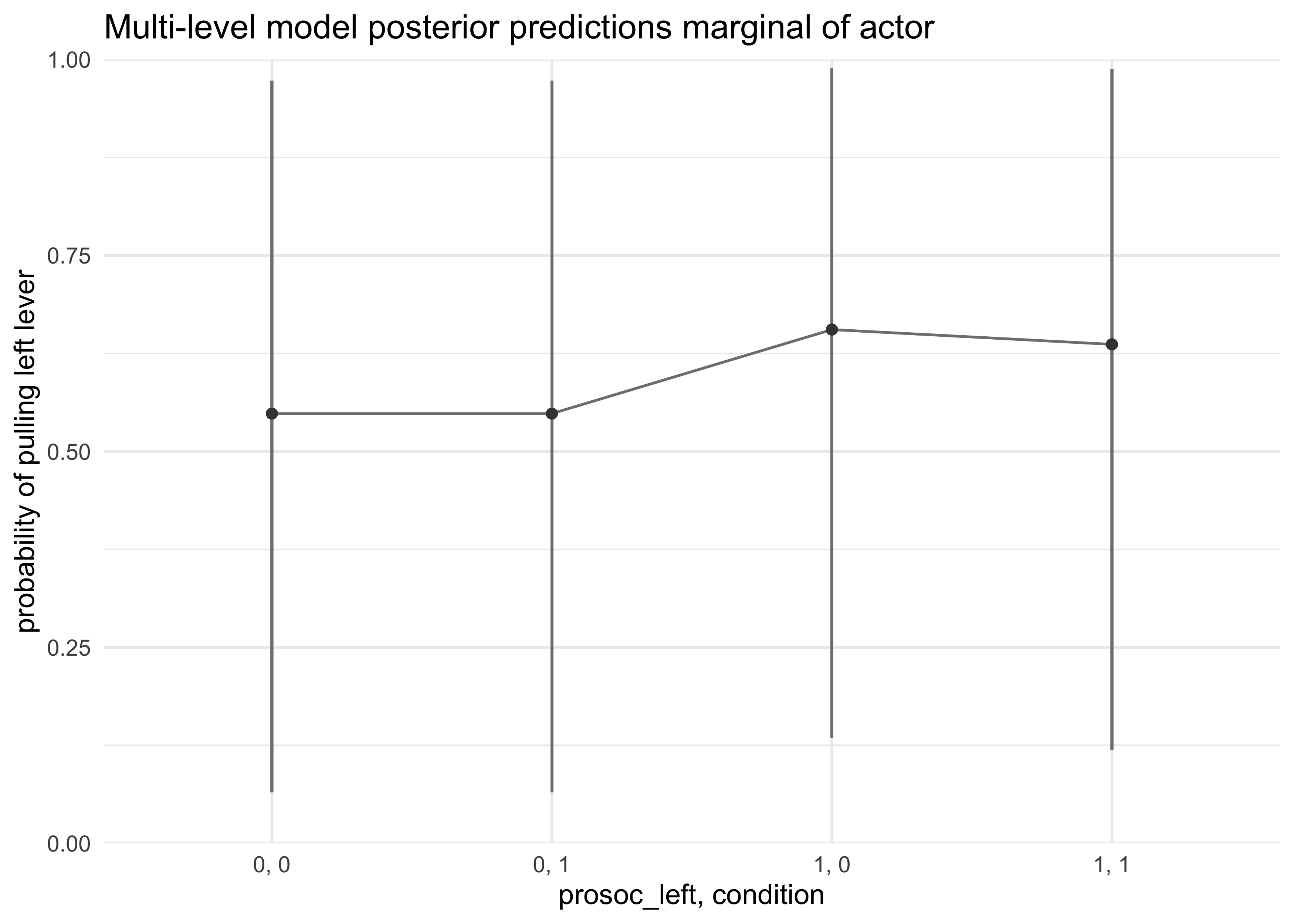
choosing which plot to use/present depends on the context and what you are trying to learn
- the average actor plot shows the effect of treatment
- the marginal of actor plot shows how variable actors can be
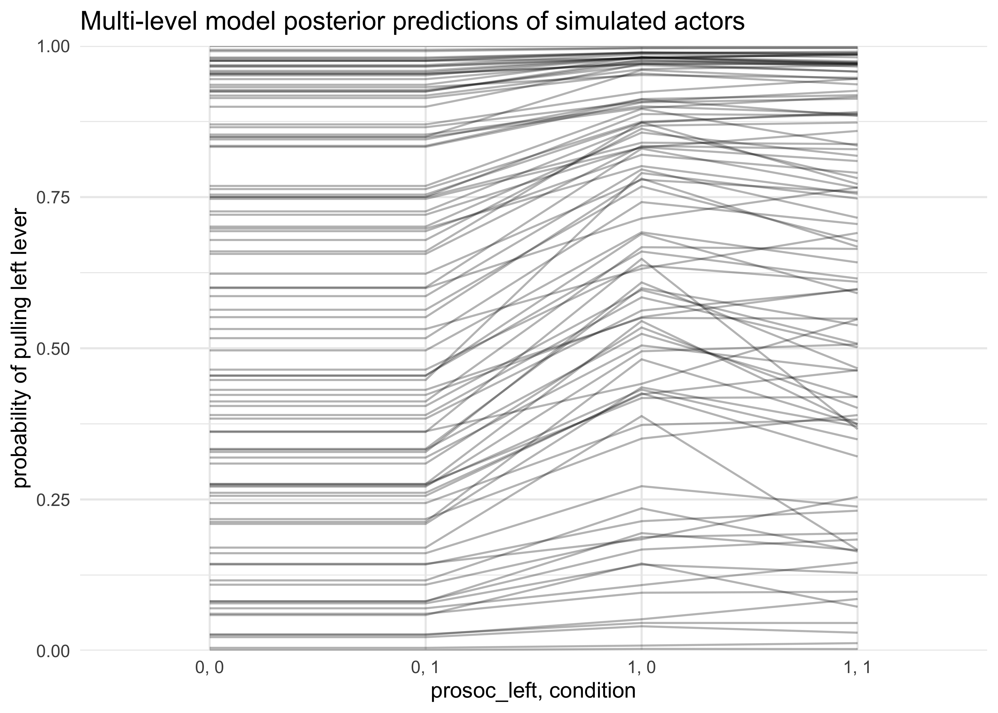
another option is to try and show both by showing the results for a bunch of new simulated actors

post <- extract.samples(m12_4, n = 1e2)
sim_actor <- function(i) {
    sim_a_actor <- rnorm(1, 0, post$sigma_actor[i])
    P <- c(0, 1, 0, 1)
    C <- c(0, 0, 1, 1)
    p <- logistic(
        post$a[i] + sim_a_actor + (post$bp[i] + post$bpc[i] * C) * P
    )
    return(
        tibble(i = i, prosoc_left = P, condition = C, pred = p)
    )
}

map_df(1:100, sim_actor) %>%
    mutate(x = paste(prosoc_left, condition, sep = ", ")) %>%
    ggplot(aes(x = x, y = pred)) +
    geom_line(aes(group = factor(i)), alpha = 0.3) +
    scale_y_continuous(limits = c(0, 1), expand = c(0, 0)) +
    labs(x = "prosoc_left, condition",
         y = "probability of pulling left lever",
         title = "Multi-level model posterior predictions of simulated actors")

12.4.3 Focus and multilevel prediction

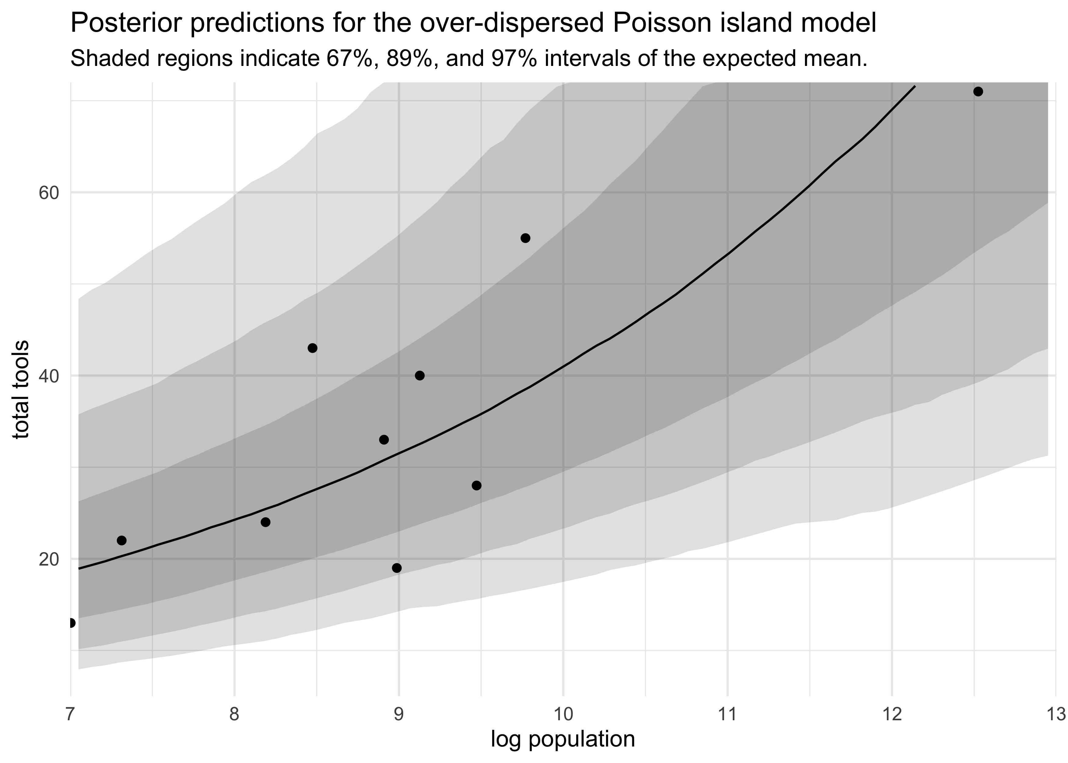
can use varying effects to model over-dispersion
- example: with Oceanic societies data with an intercept for each society
  - $T$ is the total_tools, $P$ is population, $i$ indexes each society
  - $\sigma_\text{society}$ is the estimate of over-dispersion among societies

$$ T_i \sim \text{Poisson}(\mu_i) $$ $$ \log(\mu_i) = \alpha + \alpha_{\text{society}_{[i]}} + \beta_P \log P_i $$ $$ \alpha \sim \text{Normal}(0, 10) $$ $$ \beta_P \sim \text{Normal}(0, 1) $$ $$ \alpha_\text{society} \sim \text{Normal}(0, \sigma_\text{society}) $$ $$ \sigma_\text{society} \sim \text{HalfCauchy}(0, 1) $$

data("Kline")
d <- as_tibble(Kline) %>%
    janitor::clean_names() %>%
    mutate(logpop = log(population),
           society = row_number())

stash("m12_6", {
    m12_6 <- map2stan(
        alist(
            total_tools ~ dpois(mu),
            log(mu) <- a + a_society[society] + bp * logpop,
            a ~ dnorm(0, 10),
            bp ~ dnorm(0, 1),
            a_society[society] ~ dnorm(0, sigma_society),
            sigma_society ~ dcauchy(0, 1)
        ),
        data = d,
        iter = 4e3,
        chains = 3
    )
})

#> Loading stashed object.

precis(m12_6, depth = 2)

#>                      mean         sd        5.5%       94.5%    n_eff    Rhat4
#> a              1.08087255 0.72924196 -0.10532809  2.18699862 1885.393 1.001674
#> bp             0.26289831 0.07876416  0.14412084  0.39184726 1910.748 1.001932
#> a_society[1]  -0.19505324 0.24046486 -0.59548503  0.15615568 2903.022 1.000199
#> a_society[2]   0.04898760 0.21650512 -0.28245864  0.39230167 2790.881 1.000004
#> a_society[3]  -0.03841012 0.19526471 -0.35652854  0.26649157 3589.386 1.000526
#> a_society[4]   0.33023510 0.18975208  0.05272352  0.64920133 2464.826 1.000444
#> a_society[5]   0.04739732 0.17362694 -0.22459034  0.32530026 3321.421 1.000341
#> a_society[6]  -0.31475130 0.20089950 -0.65113728 -0.01907456 3195.275 1.000715
#> a_society[7]   0.14637256 0.17070312 -0.11907974  0.42550859 3139.055 1.000605
#> a_society[8]  -0.16791652 0.17754775 -0.46365739  0.10419958 3416.196 1.001071
#> a_society[9]   0.27621050 0.17103703  0.01596246  0.55890844 2629.650 1.002193
#> a_society[10] -0.09838891 0.27906914 -0.55327144  0.32098196 2118.158 1.002263
#> sigma_society  0.30690543 0.12302611  0.14853048  0.52860652 1546.725 1.003821

plot posterior predictions that visualize the over-dispersion
- the postcheck() function uses the a_society values directly, not the hyperparameters a and sigma_society that describe the dispersion
- instead need to simulate counterfactual societies using these hyperparameters $\alpha$ and $\sigma_\text{society}$

post <- extract.samples(m12_6)

d_pred <- tibble(
    logpop = seq(6, 14, length.out = 100),
    society = rep(1, 100)
)

# Sample possible alpha society values.
a_society_sims <- rnorm(2e4, mean = 0, post$sigma_society)
a_society_sims <- matrix(a_society_sims, nrow = 2e3, ncol = 10)

# Make predictions using the simulated a_society values.
link_m12_6 <- link(m12_6, n = 2e3, data = d_pred,
                   replace = list(a_society = a_society_sims))

#> [ 200 / 2000 ][ 400 / 2000 ][ 600 / 2000 ][ 800 / 2000 ][ 1000 / 2000 ][ 1200 / 2000 ][ 1400 / 2000 ][ 1600 / 2000 ][ 1800 / 2000 ][ 2000 / 2000 ]

d_pred_res <- d_pred %>%
    mutate(mu_median = apply(link_m12_6, 2, median)) %>%
    bind_cols(
        apply(link_m12_6, 2, PI, prob = 0.67) %>% pi_to_df(),
        apply(link_m12_6, 2, PI, prob = 0.89) %>% pi_to_df(),
        apply(link_m12_6, 2, PI, prob = 0.97) %>% pi_to_df()
    )

d_pred_res %>%
    mutate(x84_percent = scales::squish(x84_percent, range = c(0, 72)),
           x94_percent = scales::squish(x94_percent, range = c(0, 72)),
           x98_percent = scales::squish(x98_percent, range = c(0, 72))) %>%
    ggplot(aes(x = logpop)) +
    geom_ribbon(aes(ymin = x2_percent, ymax = x98_percent),
                alpha = 0.15) +
    geom_ribbon(aes(ymin = x5_percent, ymax = x94_percent),
                alpha = 0.15) +
    geom_ribbon(aes(ymin = x16_percent, ymax = x84_percent),
                alpha = 0.15) +
    geom_point(aes(y = total_tools),
               data = d) +
    geom_line(aes(y = mu_median)) +
    scale_x_continuous(limits = c(7, 13), expand = c(0, 0)) +
    scale_y_continuous(limits = c(5, 72), expand = c(0, 0)) +
    labs(x = "log population",
         y = "total tools",
         title = "Posterior predictions for the over-dispersed Poisson island model",
         subtitle = "Shaded regions indicate 67%, 89%, and 97% intervals of the expected mean.")

#> Warning: Removed 36 row(s) containing missing values (geom_path).

12.6 Practice

Easy

12E2. Make the following model into a multilevel model.

$$ y_i \sim \text{Binomial}(1, p_i) $$ $$ \text{logit}(p_i) = \alpha + \alpha_{\text{group}[i]} + \beta x_i $$ $$ \alpha \sim \text{Normal}(0, 10) $$ $$ \beta \sim \text{Normal}(0, 1) $$ $$ \alpha_\text{group} \sim \text{Normal}(0, \sigma_\text{group}) $$ $$ \sigma_\text{group} \sim \text{HalfCauchy(0, 1)} $$

chapter_12