Chapter 11. Monsters And Mixtures

• build more types of models by piecing together types we have already learned about
  • will discuss ordered categorical models and zero-inflated/zero-augmented models
• mixtures are powerful, but interpretation is difficult

11.1 Ordered categorical outcomes

• the outcome is discrete and has different levels along a dimension but the differences between each level are not necessarily equal
  • is a multinomial prediction problem with a constraint on the order of the categories
  • want an estimate of the effect of a change in a predictor on the change along the categories
• use a cumulative link function
  • the cumulative probability of a value is the probability of that value or any smaller value
  • this guarantees the ordering of the outcomes

11.1.1 Example: Moral intuition

• example data come from a survey of people with different versions of the classic “Trolley problem”
  • 3 versions that invoke different moral principles: “action principle,” “intention principle,” and “contact principle”
  • the goal is how people just the different choices from the different principles
  • response: from an integer 1-7, how morally permissible is the action

data("Trolley")
d <- as_tibble(Trolley) %>%
    rename(q_case = case)

11.1.2 Describing an ordered distribution with intercepts

• some plots of the data
  • a histogram of the response values
  • cumulative proportion of responses
  • log-cumulative-odds of responses

p1 <- d %>%
    ggplot(aes(x = response)) +
    geom_histogram(bins = 30) +
    labs("Distribution of response")

p2 <- d %>% 
    count(response) %>%
    mutate(prop = n / sum(n),
           cum_prop = cumsum(prop)) %>%
    ggplot(aes(x = response, y = cum_prop)) +
    geom_line() +
    geom_point() +
    labs(y = "cumulative proportion")

p3 <- d %>% 
    count(response) %>%
    mutate(prop = n / sum(n),
           cum_prop = cumsum(prop),
           cum_odds = cum_prop / (1 - cum_prop),
           log_cum_odds= log(cum_odds)) %>%
    filter(is.finite(log_cum_odds)) %>%
    ggplot(aes(x = response, y = log_cum_odds)) +
    geom_line() +
    geom_point() +
    labs(y = "log-cumulative-odds")

p1 | p2 | p3

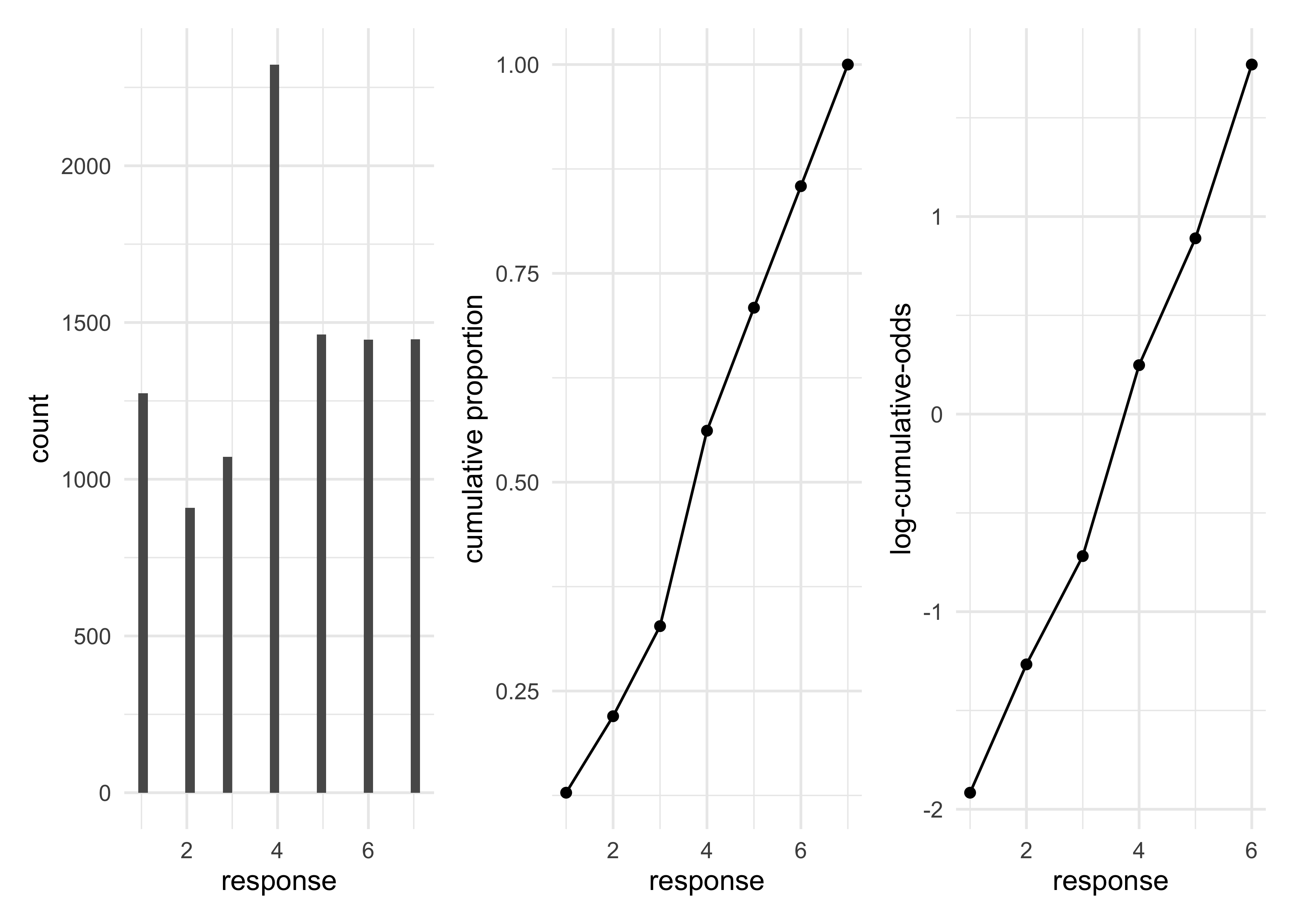
• why use the log-cumulative-odds of each response:
  • it is the cumulative analog of the logit link used previously
  • the logit is the log-odds; the cumulative logit is the log-cumulative-odds
  • constrains the probabilities to between 0 and 1
  • this link function takes care of converting the parameter estimates to the probability scale
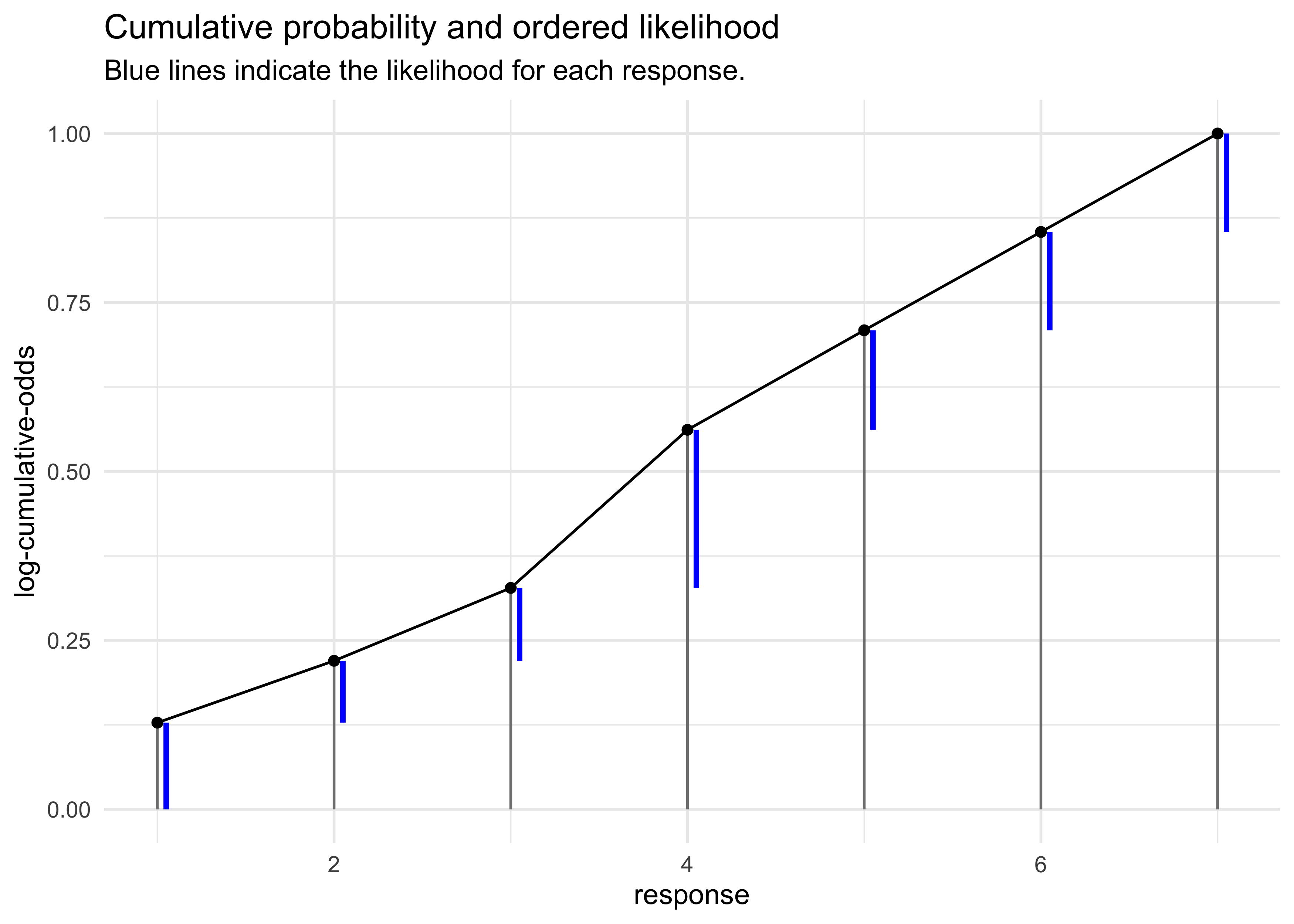
• to use Bayes’ theorom to compute the posterior distribution of these intercepts, need to compute the likelihood of each possible response value
  • need to use the cumulative probabilities $\Pr(y_i \ge k)$ to compute the likelihood $\Pr(y_i = k)$
  • use the inverse link to translate the log-cumulative-odds back to cumulative probability
  • therefore, when we observe $k$ and need its likelihoood, just use subtraction:
    • the values are shown as blue lines in the next plot

$$ p_k = \Pr(y_i = k) = \Pr(y_i \le k) - \Pr(y_i \le k - 1) $$

offset_subtraction <- function(x) {
    y <- x
    for (i in seq(1, length(x))) {
        if (i == 1) { 
            y[[i]] <- x[[i]]
        } else {
            y[[i]] <- x[[i]] - x[[i - 1]]
        }
    }
    return(y)
}

d %>% 
    count(response) %>%
    mutate(prop = n / sum(n),
           cum_prop = cumsum(prop),
           likelihood = offset_subtraction(cum_prop),
           ymin = cum_prop - likelihood) %>%
    ggplot(aes(x = response)) +
    geom_linerange(aes(ymin = 0, ymax = cum_prop), color = "grey50") +
    geom_line(aes(y = cum_prop)) +
    geom_point(aes(y = cum_prop)) +
    geom_linerange(aes(ymin = ymin, ymax = cum_prop), color = "blue",
                   position = position_nudge(x = 0.05), size = 1) +
    labs(y = "log-cumulative-odds",
         title = "Cumulative probability and ordered likelihood",
         subtitle = "Blue lines indicate the likelihood for each response.")

• below is the matematical form of the model using an ordered logit likelihood
  • notation for these models can vary by author
  • the Ordered distribution is just a categorical distribution that takes a vector $\text{p} = {p_1, p_2, p_3, p_4, p_5, p_6}$
    • only 6 because the 7th level has the value 1 automatically
  • each response value $k$ gets an intercept parameter $\alpha_k$

$$ R_i \sim \text{Ordered}(p) $$ $$ logit(P_k) = \alpha_k $$ $$ \alpha_k \sim \text{Normal}(0, 10) $$

• the first model does not include any predictor vairables
  • the link function is embedded in the likelihood function, already
    • simpler to type and makes the calculations more efficient, too
  • phi is a placeholder for now but will be used to add in predictor variables
  • the start values are included to start the intercepts in the right order
    • their exact values don’t really matter, just the order

m11_1 <- quap(
    alist(
        response ~ dordlogit(phi, c(a1, a2, a3, a4, a5, a6)),
        phi <- 0,
        c(a1, a2, a3, a4, a5, a6) ~ dnorm(0, 10)
    ),
    data = d,
    start = list(a1 = -2, a2 = -1, a3 = 0, a4 = 1, a5 = 2, a6 = 2.5)
)

precis(m11_1)

#>          mean         sd       5.5%      94.5%
#> a1 -1.9160695 0.03000701 -1.9640265 -1.8681125
#> a2 -1.2666001 0.02423126 -1.3053263 -1.2278739
#> a3 -0.7186296 0.02137978 -0.7527986 -0.6844606
#> a4  0.2477844 0.02022442  0.2154619  0.2801070
#> a5  0.8898583 0.02208975  0.8545546  0.9251620
#> a6  1.7693642 0.02845011  1.7238954  1.8148329

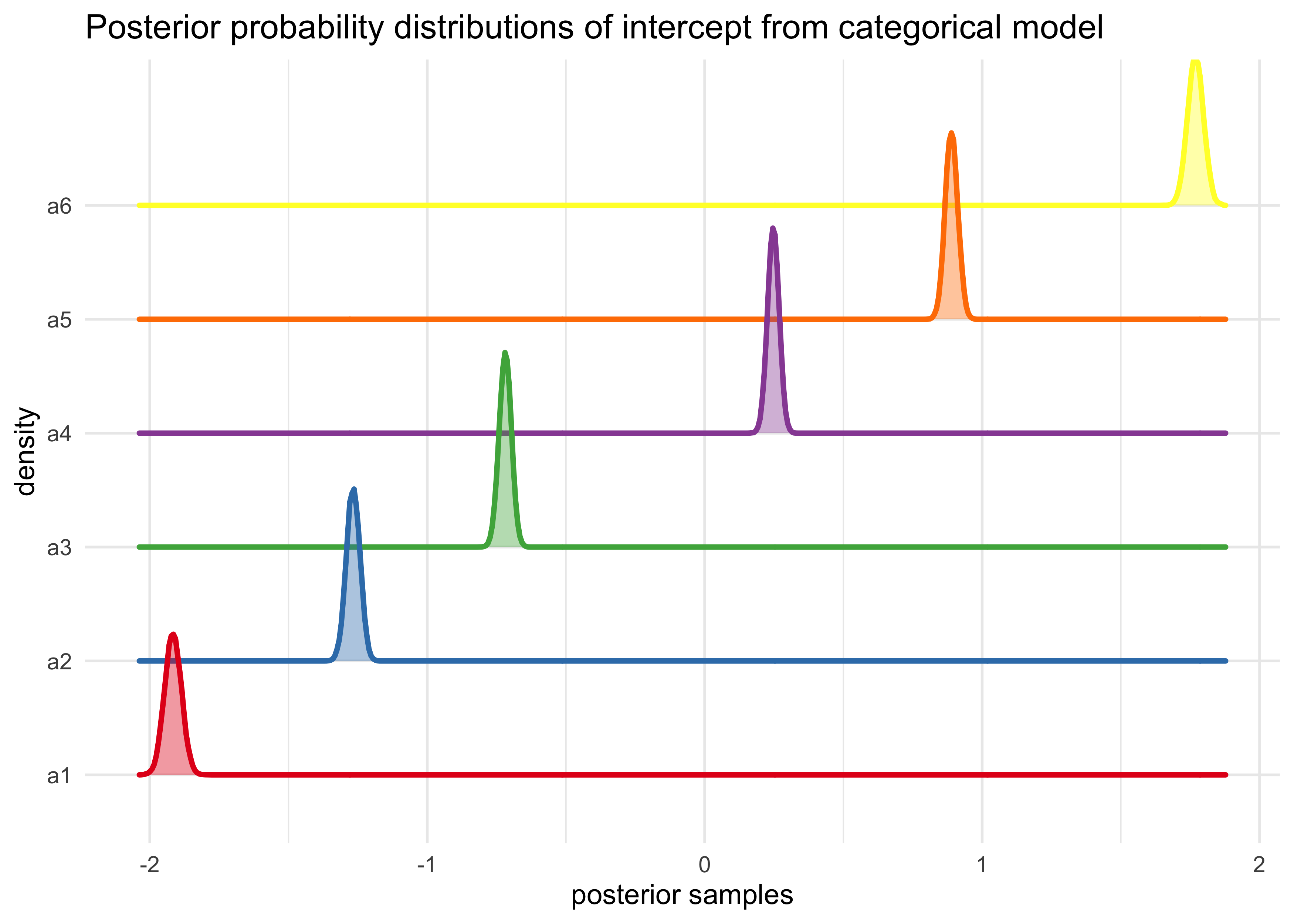
• transform from log-cumulative-odds to cumulative probabilities

logistic(coef(m11_1))

#>        a1        a2        a3        a4        a5        a6 
#> 0.1283005 0.2198398 0.3276948 0.5616311 0.7088609 0.8543786

m11_1_link <- extract.samples(m11_1)
m11_1_link %>%
    as.data.frame() %>%
    as_tibble() %>%
    pivot_longer(tidyselect::everything()) %>%
    ggplot(aes(x = value, y = name, color = name, fill = name)) +
    ggridges::geom_density_ridges(size = 1, alpha = 0.4, ) +
    scale_color_brewer(palette = "Set1") +
    scale_fill_brewer(palette = "Set1") +
    theme(legend.position = "none") +
    labs(x = "posterior samples",
         y = "density",
         title = "Posterior probability distributions of intercept from categorical model")

#> Picking joint bandwidth of 0.00348

11.1.3 Adding predictor variables

• to include predictor variables:
  • define the log-cumulative-odds of each response $k$ as a sum of its intercept $\alpha_k$ and a typical linear model
  • for example: add a predictor $x$ to the model
    • define the linear model $\phi_i = \beta x_i$
    • the cumulative logit becomes:

$$ \log \frac{\Pr(y_i \ge k)}{1 - \Pr(y_i \ge k)} = \alpha - \phi_i = \alpha - \beta x_i $$

• this form keeps the correct ordering of the outcome values while still morphing the likelihood of each individual value as the predictor $x_i$ changes value
• the linear model $\phi$ is subtracted from the intercept:
  • because decreasing the log-cumulative-odds of every outcome value $k$ below the maximum shifts probability mass upwards towards higher outcome values
  • a positive $\beta$ value indicates than an increase in the predictor variable $x$ results in an increase in the average response
• for the Trolly data, we can icnlude predictor variables for the different types of questions: “action,” “intention,” and “contact”
  • the formulation of the log-cumulative-odds of each response $k$ is shown below
  • defines the log-odds of each possible response to be an additive model of the features of the story corresponding to each response

$$ \log \frac{\Pr(y_i \ge k)}{1 - \Pr(y_i \ge k)} = \alpha - \phi_i $$ $$ \phi_i = \beta_A A_i + \beta_I I_i + \beta_C C_i $$

m11_2 <- quap(
    alist(
        response ~ dordlogit(phi, c(a1, a2, a3, a4, a5, a6)),
        phi <- bA*action + bI*intention + bC*contact,
        c(a1, a2, a3, a4, a5, a6) ~ dnorm(0, 10),
        c(bA, bI, bC) ~ dnorm(0, 10)
    ),
    data = d,
    start = list(a1 = -2, a2 = -1, a3 = 0, a4 = 1, a5 = 2, a6 = 2.5)
)

• fit another model with interactions between action and intention and between contact and intention
  • these two make sense in terms of the scenario we are modeling while an interaction between contact and action does not
    • contact is a type of action

m11_3 <- quap(
    alist(
        response ~ dordlogit(phi, c(a1, a2, a3, a4, a5, a6)),
        phi <- bA*action + bI*intention + bC*contact + bAI*action*intention + bCI*contact*intention,
        c(a1, a2, a3, a4, a5, a6) ~ dnorm(0, 10),
        c(bA, bI, bC, bAI, bCI) ~ dnorm(0, 10)
    ),
    data = d,
    start = list(a1 = -2, a2 = -1, a3 = 0, a4 = 1, a5 = 2, a6 = 2.5)
)

coeftab(m11_1, m11_2, m11_3)

#>      m11_1   m11_2   m11_3  
#> a1     -1.92   -2.84   -2.63
#> a2     -1.27   -2.15   -1.94
#> a3     -0.72   -1.57   -1.34
#> a4      0.25   -0.55   -0.31
#> a5      0.89    0.12    0.36
#> a6      1.77    1.02    1.27
#> bA        NA   -0.71   -0.47
#> bI        NA   -0.72   -0.28
#> bC        NA   -0.96   -0.33
#> bAI       NA      NA   -0.45
#> bCI       NA      NA   -1.27
#> nobs    9930    9930    9930

• interpretation:
  • the intercepts are difficult to interpret on their own, but act like regular intercepts in simpler models
    • they are the relative frequencies of the outcomes when all predictors are set to 0
  • there are 5 slope parameters: 3 main effects and 2 iinteractions
    • they are all far from 0 (can check with precis(m))
    • they are all negative: each factor/interaction reduces the average response
    • these values are difficult to interpret as is, so they are investigated more below
• compare the models by WAIC
  • the model with interaction terms is sufficiently better than the other two, so we can safely proceed with just analyzing it and ignoring the other two

compare(m11_1, m11_2, m11_3)

#>           WAIC       SE    dWAIC      dSE     pWAIC        weight
#> m11_3 36929.15 81.16718   0.0000       NA 11.004379  1.000000e+00
#> m11_2 37090.36 76.34564 161.2159 25.78738  9.253143  9.826897e-36
#> m11_1 37854.49 57.63045 925.3444 62.65109  6.020406 1.158826e-201

• plot implied predictions to understand what model m11_3 implies
  • difficult to plot the predictions of log-cumulative-odds because each prediction is a vector of probabilities, one for each possible outcome
  • as a predictor variable changes value, the entire vector changes
• one common plot is to use the horiztonal axis for the predictor variable and the vertical axis for the cumulative probability
  • plot a curve for each response value

post <- extract.samples(m11_3)

get_m11_3_predictions <- function(kA, kC, kI) {
    res <- tibble()
    for (s in 1:100) {
        p <- post[s, ]
        ak <- as.numeric(p[1:6])
        phi <- p$bA * kA + p$bI*kI + p$bC*kC + p$bAI*kA*kI + p$bCI*kC*kI
        pk <- pordlogit(1:6, a = ak, phi = phi)
        res <- bind_rows(
            res,
            tibble(lvl = 1:6, val = pk)
        )
    }
    return(res)
}


implied_predictions <- expand.grid(kA = 0:1, kC = 0:1, kI = 0:1) %>%
    as_tibble() %>%
    filter(!(kA == 1 & kC == 1)) %>% 
    group_by(kA, kC, kI) %>%
    mutate(preds = list(get_m11_3_predictions(kA, kC, kI))) %>%
    unnest(preds) %>%
    ungroup()

implied_predictions %>%
    mutate(facet = paste0("action: ", kA, ", ", "contact: ", kC)) %>%
    group_by(kA, kC, kI) %>%
    mutate(row_idx = row_number()) %>%
    ungroup() %>%
    mutate(line_group = paste(lvl, row_idx)) %>%
    ggplot(aes(x = kI, y = val, group = line_group)) +
    facet_wrap(~ facet, nrow = 1) +
    geom_hline(yintercept = 0:1, lty = 2, color = "grey70", size = 1) +
    geom_line(aes(color = factor(lvl)), alpha = 0.1) +
    scale_color_brewer(palette = "Dark2") +
    labs(x = "intention", 
         y = "probability",
         color = "level",
         title = "Implied predictions of model with interactions.")

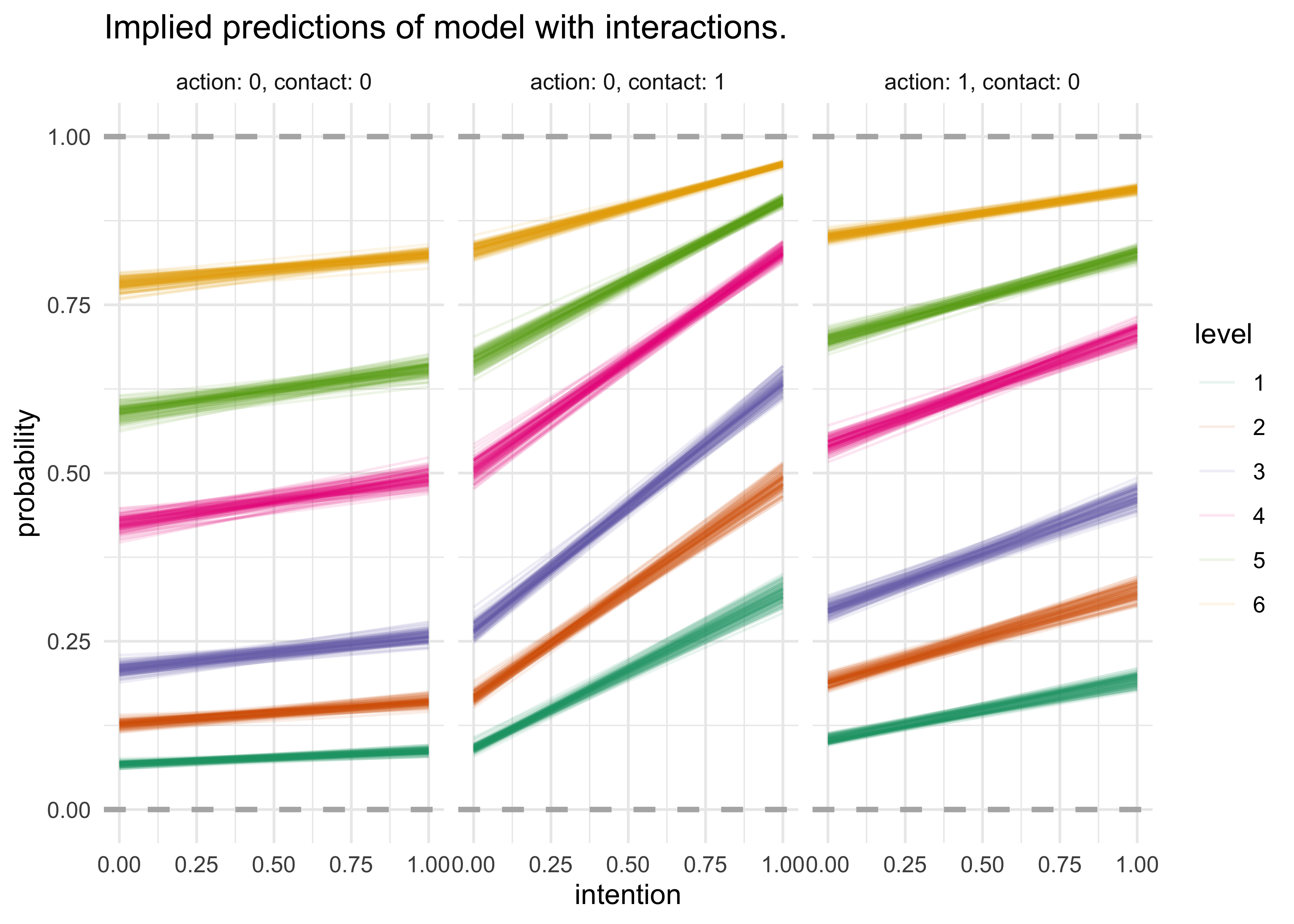
• interpretation:
  • each horizontal line is the bounday between levels
  • the thickness of the boundary represents the variation in prediction
  • the change in height from intention changing from 0 to 1 indicates the predicted impact of changing a trolley story from non-intention to intention
    • the left-hand plot shows that there is not much change from switching intention when action and contact are both 0
    • the other two plots show the interaction between intention and the other variable that is set to 1
    • the middle plot shows that there is a large interaction between contact and intention

11.2 Zero-inflated outcomes

• mixture model: measurements arise from multiple proceesses; different causes for the same observation
  • uses more than one probability distribution
• common to need to use a mixture model for count variables
  • a count of 0 can often arise in more than one way
  • a 0 could occurr because nothing happens, because the rate of the event is very low, or because the event-generating process never began
  • said to be zero-inflated

11.2.1 Example: Zero-inflated Poisson

• previously, we use the monastery example to study the Poisson distribution
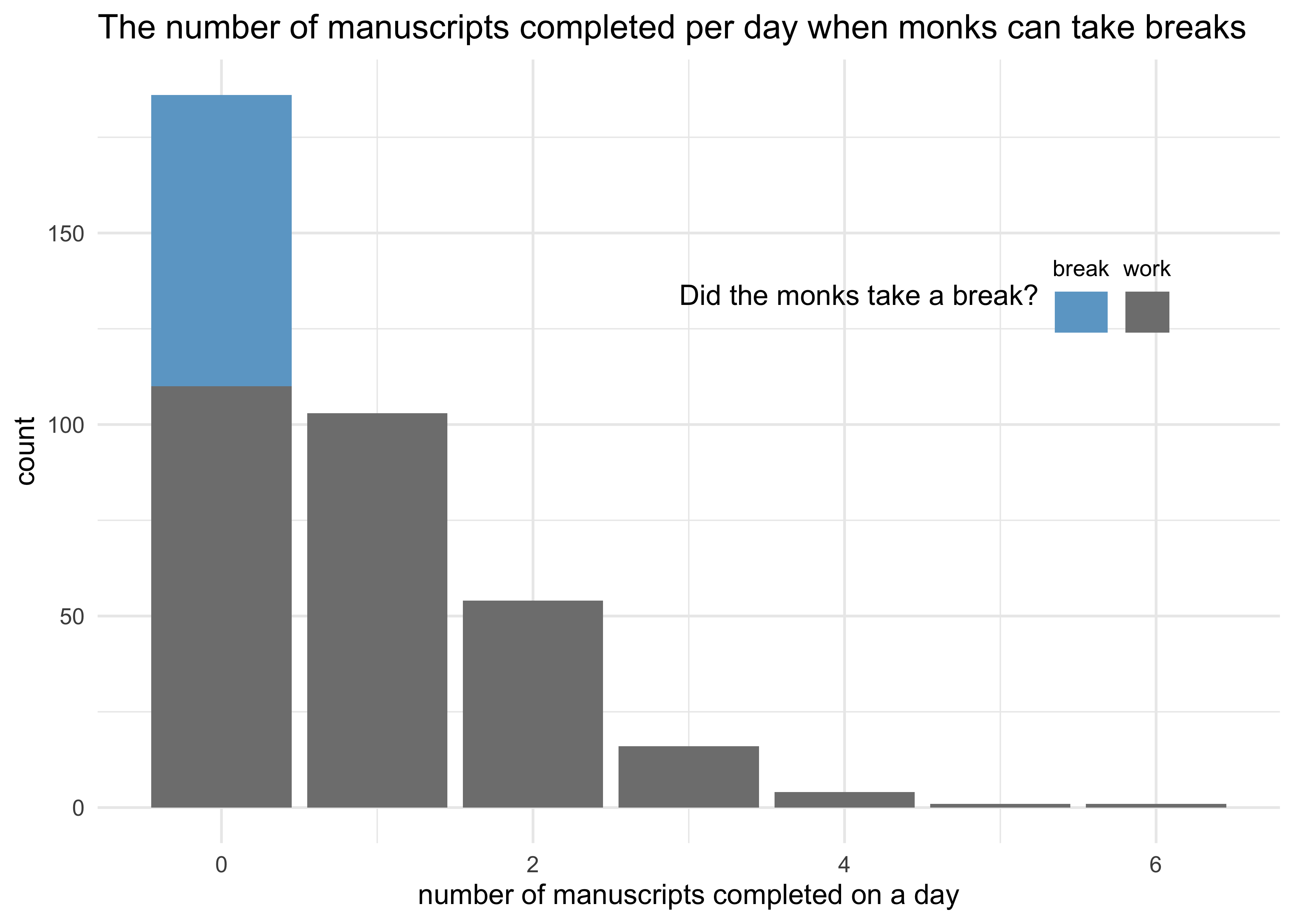
  • now imagine that the monks take breaks on some days and no manuscripts are made
  • want to estimate how often breaks are taken
• mixture model:
  • a zero can arise from two processes:
    1. the monks took a break
    2. the monks workked but did not complete a manuscript
  • let $p$ be the probability the monks took a break on a day
  • let $\lambda$ be the mean number of manuscripts completed when the monks work
• need a likelihood function that mixes these two processes:
  • the following equation says this: “The probability of observing a zero is the probability that the monks took a break OR ($+$) the probability the monks worked AND ($\times$) failed to finish.”

$$ \Pr(0 | p, \lambda) = \Pr(\text{break} | p) + \Pr(\text{work} | p) \times \Pr(0 | \lambda) $$ $$ \Pr(0 | p, \lambda) = p + (1-p) e^{-\lambda} $$

• the likelihood of a non-zero value $y$ is below
  • the the probability that the monks work multiplied by the probability that the working monks produce a manuscript

$$ \Pr(y | p, \lambda) = \Pr(\text{break} | p)(0) + \Pr(\text{work} | p) \Pr(y | \lambda) $$ $$ \Pr(y | p, \lambda) = (1 - p) \frac{\lambda^y e^{-\lambda}}{y!} $$

• can define ZIPoisson as the distribution above with parameters $p$ (probability of 0) and $\lambda$ (mean of Poisson) to describe the shape
  • two linear models and two link functions, one for each process

$$ y_i \sim \text{ZIPoisson}(p_i, \lambda_i) $$ $$ \text{logit}(p_i) = \alpha_p + \beta_p x_i $$ $$ \log(\lambda_i) = \alpha_\lambda + \beta_\lambda x_i $$

• need to simulate data for the monks taking breaks

# They take a break on 20% of the days
prob_break <- 0.2 

# Average of 1 manuscript per working day.
rate_work <- 1

# Sample one year of production.
N <- 365

# Simulate which days the monks take breaks.
break_days <- rbinom(N, 1, prob = prob_break)

# Simulate the manuscripts completed.
y <- (1-break_days) * rpois(N, rate_work)

tibble(y, break_days) %>%
    count(y, break_days) %>%
    mutate(break_days = ifelse(break_days == 0, "work", "break"),
           break_days = factor(break_days, levels = c("break", "work"))) %>%
    ggplot(aes(x = y, y = n)) +
    geom_col(aes(fill = break_days)) +
    scale_fill_manual(
        values = c("skyblue3", "grey50"),
        guide = guide_legend(title.position = "left",
                             title.hjust = 0.5,
                             label.position = "top",
                             ncol = 2)
    ) +
    theme(
        legend.position = c(0.7, 0.7)
    ) +
    labs(x = "number of manuscripts completed on a day",
         y = "count",
         fill = "Did the monks take a break?",
         title = "The number of manuscripts completed per day when monks can take breaks")

• now we can fit a model

m11_4 <- quap(
    alist(
        y ~ dzipois(p, lambda),
        logit(p) <- ap,
        log(lambda) <- al,
        ap ~ dnorm(0, 1),
        al ~ dnorm(0, 10)
    ),
    data = tibble(y)
)

precis(m11_4)

#>           mean         sd        5.5%      94.5%
#> ap -1.08474003 0.27298308 -1.52101972 -0.6484603
#> al  0.04329227 0.08613731 -0.09437178  0.1809563

logistic(m11_4@coef[["ap"]])

#> [1] 0.2526101

exp(m11_4@coef[["al"]])

#> [1] 1.044243

• can get a very accurate prediction for the proportion of days taken off by the monks and the rate of manuscript production per working day
  • though, cannot determine whether the monks took any particular day off

11.3 Over-dispersed outcomes

• over-dispersion: the variance of a variable exceededs the expected amount for a model
  • e.g.: for a binomial, the expected value is $np$ and its variance $np(1-p)$
  • for a count model, this suggests that a necessary variable has been omitted
• ideally, would just include the missing variable to remove over-dispersion, but not always the case/possible
• two strategies for mitigating the effects of over-dispersion
  • use a continuous mixture model: a linear model is attached to a distribution of observations
    • common models: beta-binomial and gamma-Poisson (negative-binomial)
    • these are demonstrated in the following sections
  • employ a multilevel model (GLMM) and estimate the residuals of each observation and the distribution of those residuals
    • easier to fit than beta-binmial and gamma-Poisson GLMs
    • more flexible
    • handle over-dispersion and other kinds of heterogineity simulatneously
    • GLMMs are covered in the next chapter

11.3.1 Beta-binomial

• beta-binomial models assumes that each binomial count observation has its own probability of a success
  • estimates the distribution of probabilities of success across cases
    • instead of a single probability of success
  • predictor variables change the shape of this distribution instead of directly determining the probability of each success
• example: UCB admissions data
  • if we ignore the department, the data is very over-dispersed
    • because the departments vary a lot in baseline admission rates
  • therefore, ignoring the inter-department variation results in an incorrect inference about applicant gender
  • can fit a beta-binomial model, ignoring department
• a beta-binomial model will assume that each row of the data has a unique, unobserved probability of admission
  • these probabilities of admission have a common distribution described by the beta distribution
    • use the beta distribution because it can be used to calculate the likelihood function that averages over the unknown probabilities for each observation
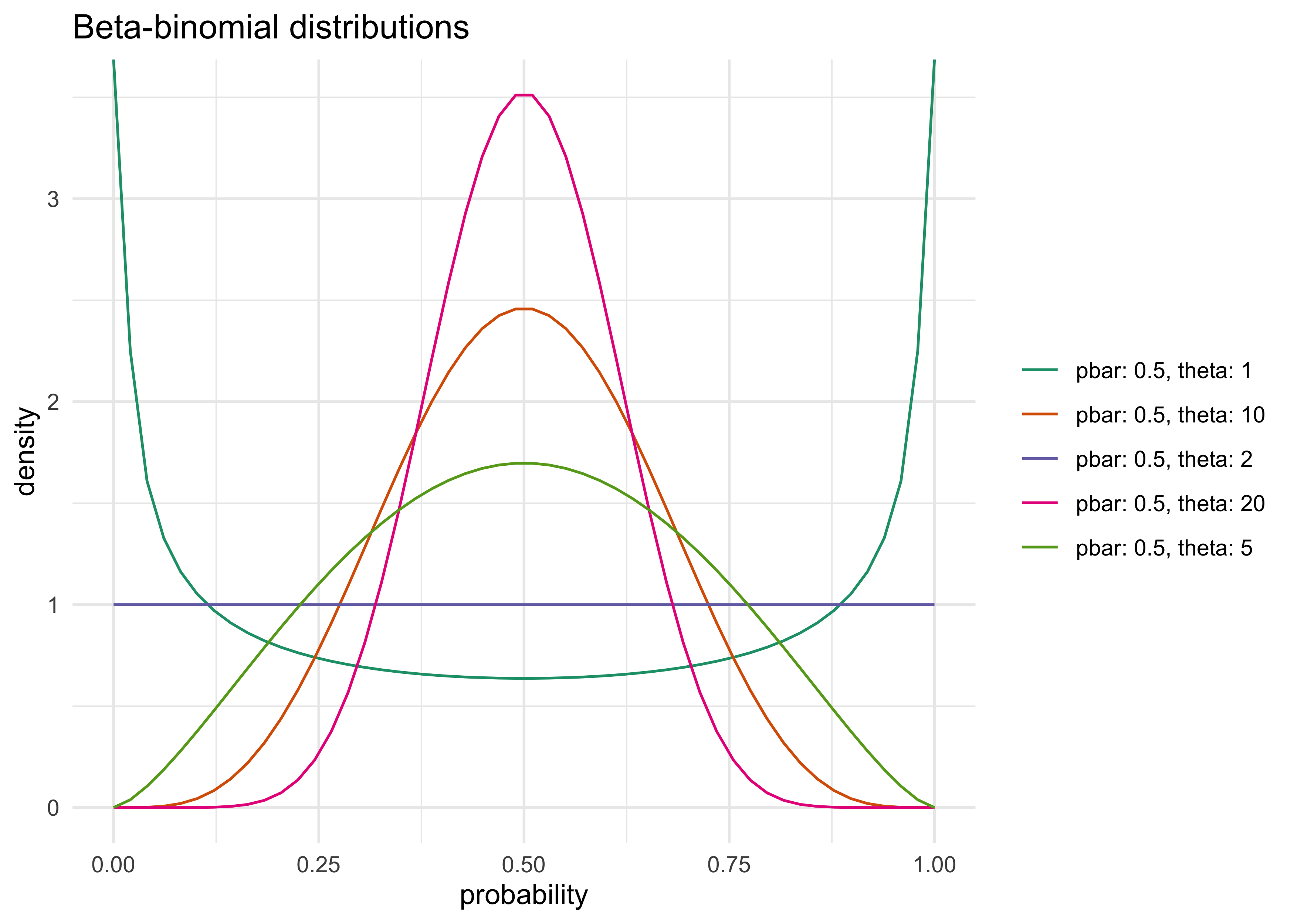
  • beta-distribution has 2 parameters:
    1. $\bar{\textbf{p}}$: average probability
    2. $\theta$: shape parameter
  • shape parameter describes the spread of the distribution

pbar <- 0.5
thetas <- c(1, 2, 5, 10, 20)
x_vals <- seq(0, 1, length.out = 50)
beta_dist_res <- tibble()
for (theta in thetas) {
    beta_dist_res <- bind_rows(
        beta_dist_res,
        tibble(theta = theta, 
               pbar = pbar, 
               x = x_vals,
               d = dbeta2(x_vals, pbar, theta))
    )
}

beta_dist_res %>%
    mutate(params = paste0("pbar: ", pbar, ", theta: ", theta)) %>%
    ggplot(aes(x = x, y = d)) +
    geom_line(aes(group = params, color = params)) +
    scale_color_brewer(palette = "Dark2") +
    labs(x = "probability", y = "density", color = NULL,
         title = "Beta-binomial distributions")

• we will build a linear model to $\bar{\textbf{p}}$ so that changes in predictor variables change the central tendency of the distribution
  • $A$ is the number of admissions (admit column)
  • $n$ is the number of applications (applications column)
  • any predictor variables could be included in the linear model for $\bar{p}$

$$ A_i \sim \text{BetaBinomial}(n_i, \bar{p}_i, \theta) $$ $$ \text{logit}(\bar{p}_i) = \alpha $$ $$ \alpha \sim \text{Normal}(0, 10) $$ $$ \theta \sim \text{HalfCauchy}(0, 1) $$

data("UCBadmit")
d <- as_tibble(UCBadmit) %>%
    janitor::clean_names()

stash("m11_5", depends_on = "d", {
    m11_5 <- map2stan(
        alist(
            admit ~ dbetabinom(applications, pbar, theta),
            logit(pbar) <- a,
            a ~ dnorm(0, 2),
            theta ~ dexp(1)
        ),
        data = d,
        constraints = list(theta = "lower=0"),
        start = list(theta = 3),
        iter = 4e3, 
        warmup = 1e3, 
        chains = 2, 
        cores = 1
    )
})

#> Loading stashed object.

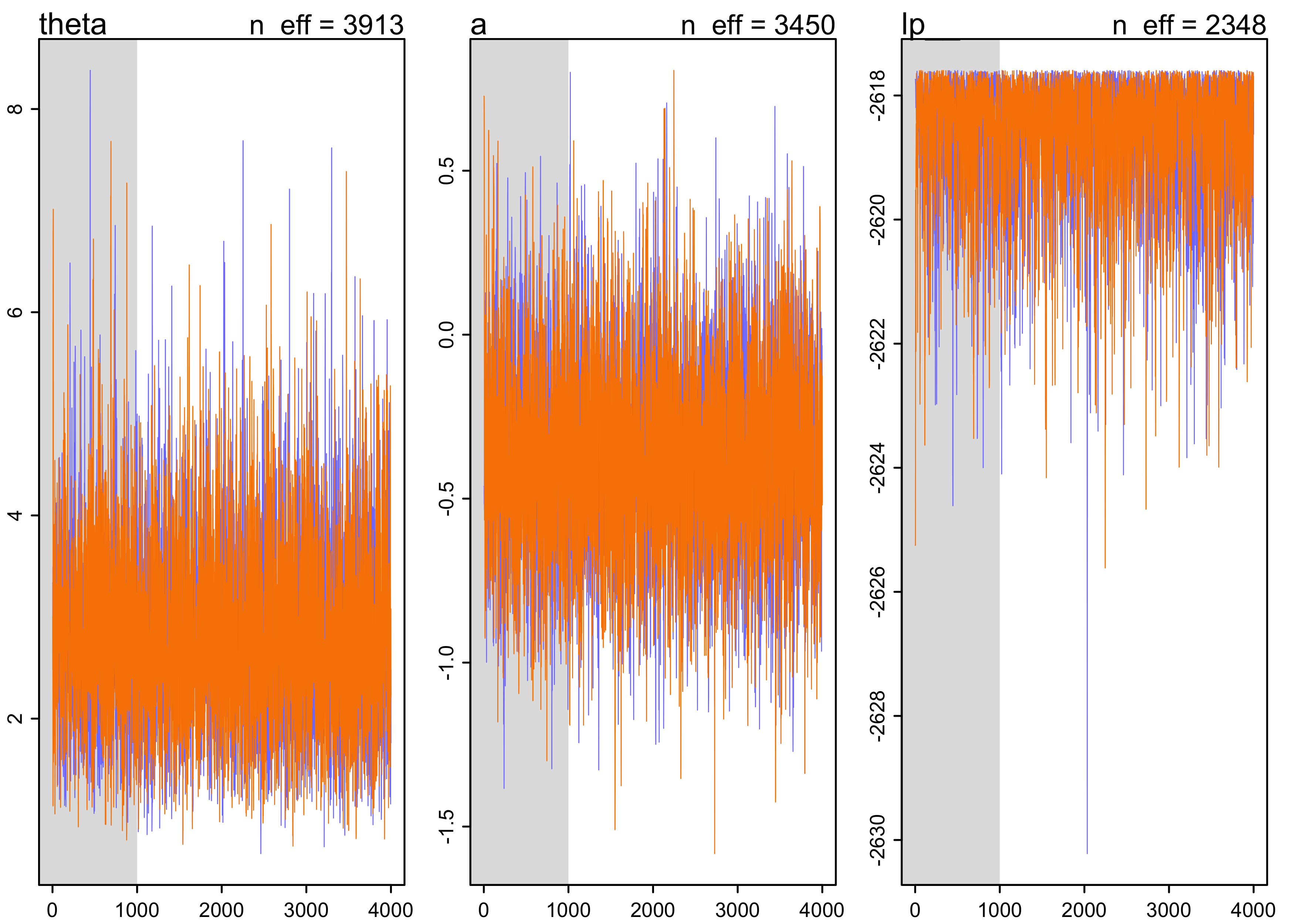
plot(m11_5)

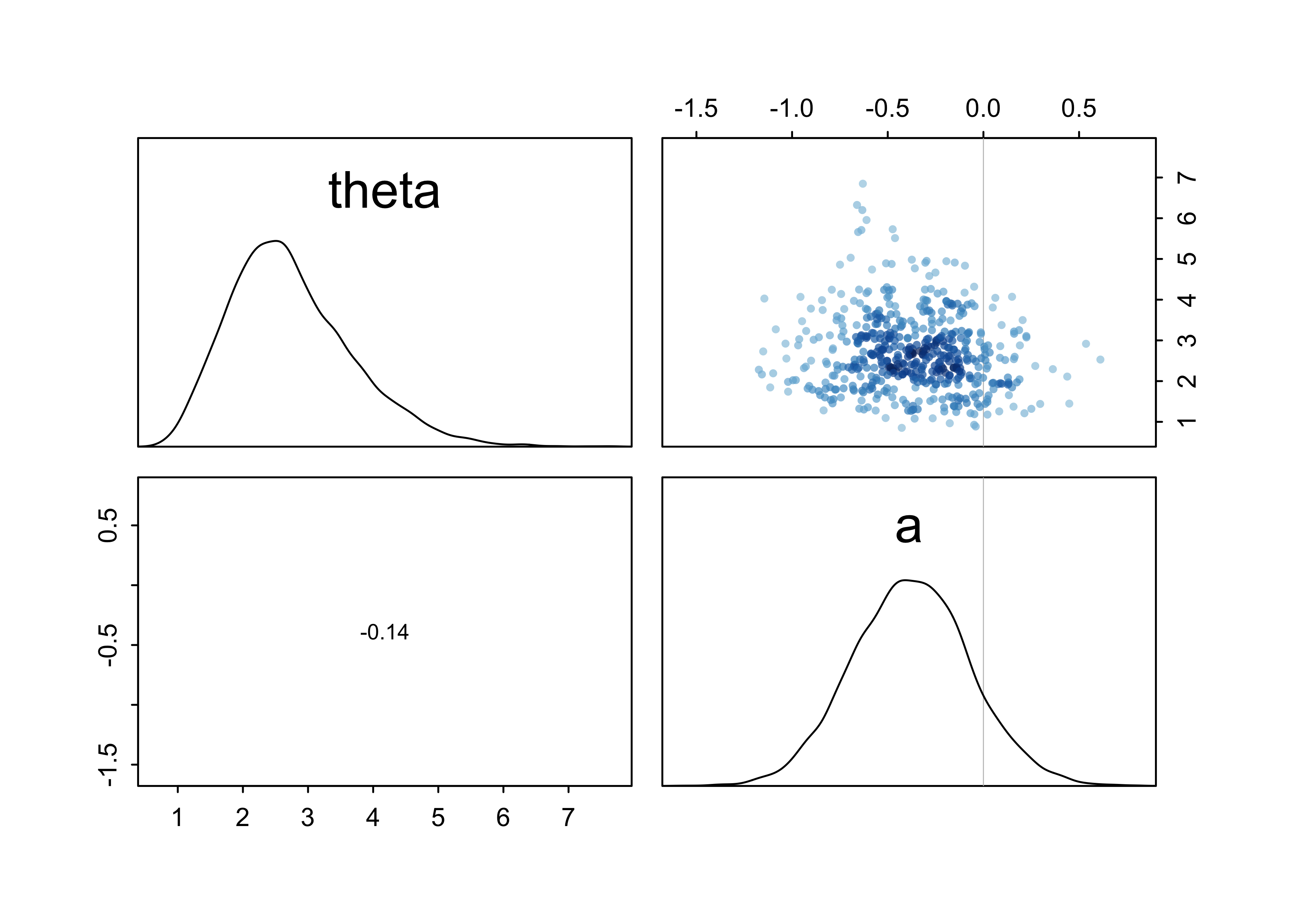
pairs(m11_5)

precis(m11_5)

#>             mean       sd       5.5%     94.5%    n_eff     Rhat4
#> theta  2.7399242 0.946932  1.4355572 4.4392494 3913.286 0.9997085
#> a     -0.3775653 0.307988 -0.8717805 0.1203542 3450.286 1.0000152

• interpretation:
  • a is on the log-odds scale and defines $\bar{\textbf{p}}$ of the beta distribution of probabilities for each row of the data
  • therefore, the average probability of admission across departments is about 0.4, but the percentile is quite wide

post <- extract.samples(m11_5)
quantile(logistic(post$a), c(0.025, 0.5, 0.975))

#>      2.5%       50%     97.5% 
#> 0.2749293 0.4066962 0.5588299

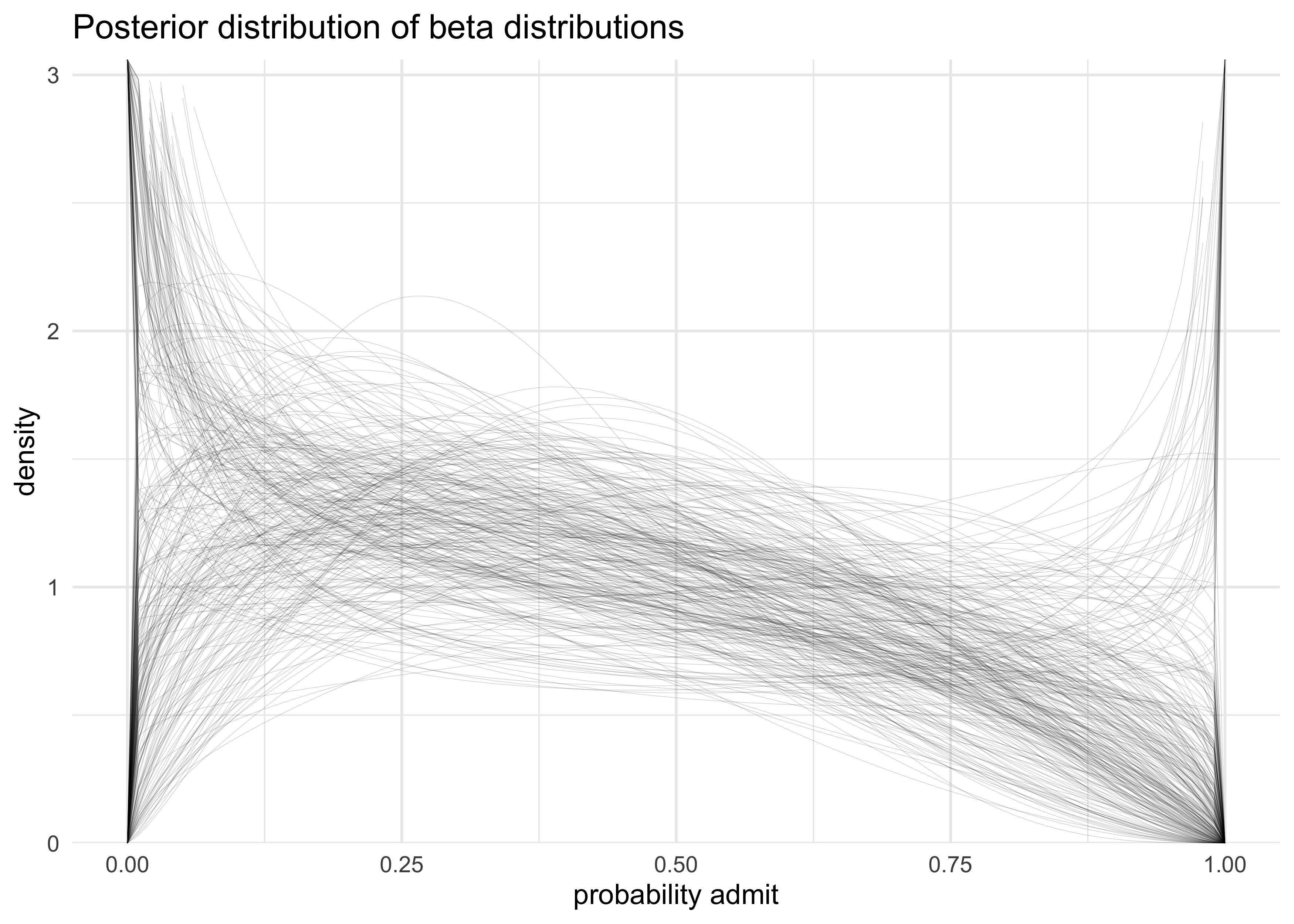
• to see what the model says of the data, need to account for correlation between $\bar{\textbf{p}}$ and $\theta$
  • these parameters define a distribution of distributions
  • 100 combinations of $\bar{\textbf{p}}$ and $\theta$ are shown in the following plot

dist_of_dist <- map(1:300, function(i) {
    p <- logistic(post$a[i])
    theta <- post$theta[i]
    x <- seq(0, 1, length.out = 100)
    probs <- dbeta2(x, p, theta)
    return(tibble(i, p, theta, x, prob = probs))
}) %>%
    bind_rows()

dist_of_dist %>%
    ggplot(aes(x, prob)) +
    geom_line(aes(group = factor(i)), size = 0.1, alpha = 0.2) +
    scale_y_continuous(limits = c(0, 3), 
                       expand = expansion(mult = c(0, 0.02))) +
    labs(x = "probability admit", 
         y = "density",
         title = "Posterior distribution of beta distributions")

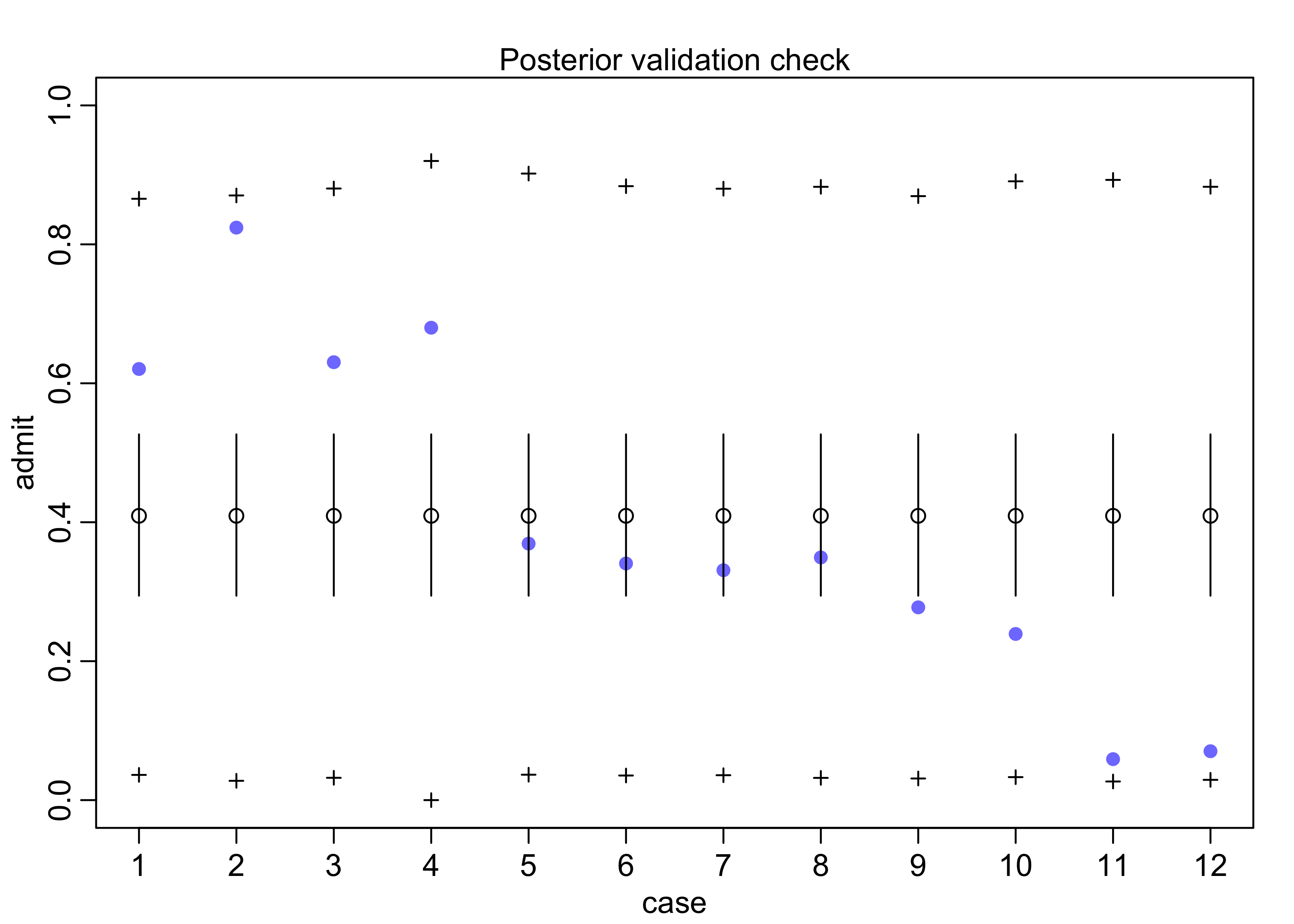
• use posterior check to see how the beta distribution of probabilities of admissions influences predicted counts of applications admitted
  • the y-axis shows the predicted number of admits per row of the data frame on the x-axis
  • the purple dots are the actual values
  • open circles are the estimates from the model with 89% intervals
  • the + are the 89% interval of predicted counts of admission
    • shows there is a lot of dispersion
    • this is from the different departments, but the model doesn’t know about them
    • the beta distribution accounts for this heterogeneity

postcheck(m11_5)

#> [ 100 / 1000 ][ 200 / 1000 ][ 300 / 1000 ][ 400 / 1000 ][ 500 / 1000 ][ 600 / 1000 ][ 700 / 1000 ][ 800 / 1000 ][ 900 / 1000 ][ 1000 / 1000 ]
#> [ 100 / 1000 ][ 200 / 1000 ][ 300 / 1000 ][ 400 / 1000 ][ 500 / 1000 ][ 600 / 1000 ][ 700 / 1000 ][ 800 / 1000 ][ 900 / 1000 ][ 1000 / 1000 ]

11.3.2 Negative-binomial or gamma-Poisson

• negative-binomial (or gamma-Poisson): assumes that each Poisson count observation has its own rate
  • assumes the shape of the gamma distribution to describe the Poisson rates
  • predictor variables adjust the shape of this distribution, not the expected value of each observation
  • use the gamma distribution because it makes the math easier
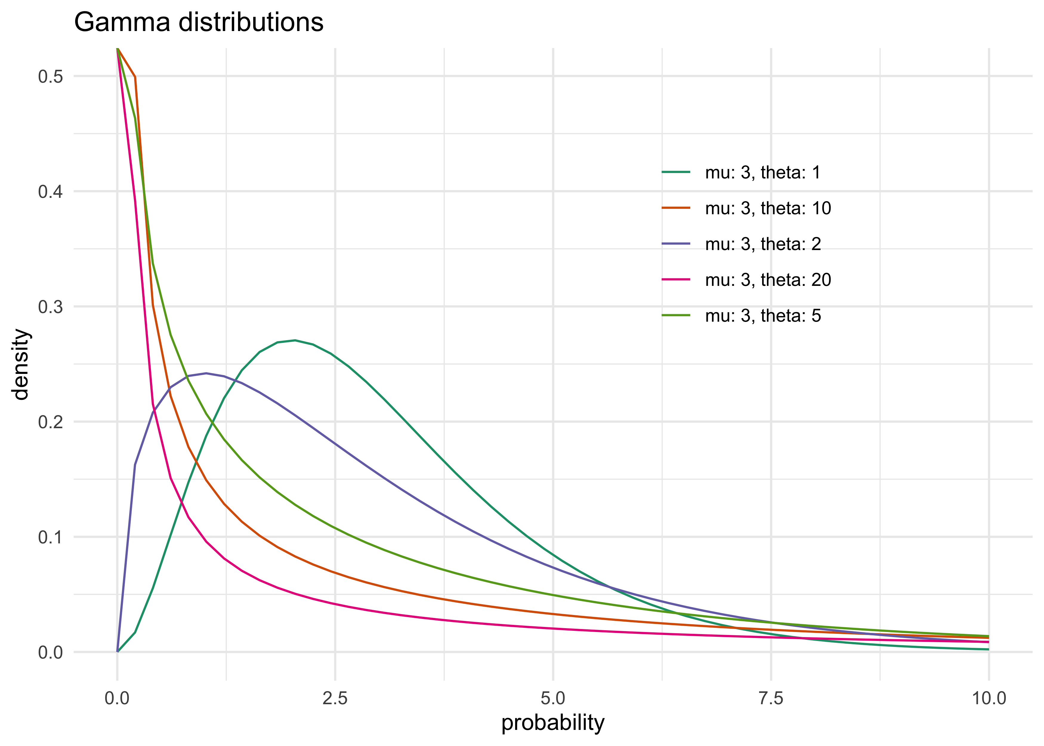
• fitting a gamma-Poisson uses the dgampois() function
  • distribution is defined by a mean $\mu$ and scale $\theta$
  • as $\theta$ increases, the gamma distribution becomes for dispersed around the mean
• below are some examples of gamma distributions
  • as $\theta$ approaches 0, the gamma approaches a Gaussian

mu <- 3
thetas <- c(1, 2, 5, 10, 20)
x_vals <- seq(0, 10, length.out = 50)
gamma_dist_res <- tibble()
for (theta in thetas) {
    gamma_dist_res <- bind_rows(
        gamma_dist_res,
        tibble(theta, 
               mu,
               x = x_vals,
               d = dgamma2(x_vals, mu, theta))
    )
}

gamma_dist_res %>%
    mutate(params = paste0("mu: ", mu, ", theta: ", theta)) %>%
    ggplot(aes(x = x, y = d)) +
    geom_line(aes(group = params, color = params)) +
    scale_color_brewer(palette = "Dark2") +
    theme(
        legend.position = c(0.7, 0.7)
    ) +
    labs(x = "probability", y = "density", color = NULL,
         title = "Gamma distributions")

• for fitting:
  • a linear model can be attached to the definition of $\mu$ using the log link function
  • there are examples in ?dgampois and practice problems at the end of the chapter

11.3.3 Over-dispersion, entropy, and information criteria

• should use DIC instead of WAIC
  • see text for an explination of why